Goodness of fit

A divergence tells you how far two models are apart; goodness-of-fit diagnostics tell you how well a model matches data. This tutorial builds the standard univariate toolkit — QQ plots, empirical-vs-fitted CDF overlays, and Kolmogorov–Smirnov tests — and applies it to synthetic and real return series.

import jax
jax.config.update("jax_enable_x64", True)
import jax.numpy as jnp
import numpy as np
import pandas as pd
from pathlib import Path
from scipy import stats

from normix import NormalInverseGaussian, UnivariateNormalInverseGaussian
from normix.utils.plotting import set_theme

set_theme()

Fitting a univariate model

Multivariate marginals are fit on (n, 1) data; we then read off the scalar parameters into a Univariate* object, which adds the cdf and ppf needed for tail diagnostics:

def fit_univariate_nig(x, **fit_kwargs):
    """Fit a 1-D NIG and return a UnivariateNormalInverseGaussian."""
    X = jnp.asarray(x, dtype=jnp.float64).reshape(-1, 1)
    m = NormalInverseGaussian.default_init(X).fit(X, **fit_kwargs).model
    return UnivariateNormalInverseGaussian.from_classical(
        mu=float(m.mu[0]), gamma=float(m.gamma[0]),
        sigma=float(m.sigma()[0, 0]), mu_ig=float(m.mu_ig), lam=float(m.lam))

Synthetic check

We draw from a known univariate NIG, refit, and confirm the diagnostics pass:

truth = UnivariateNormalInverseGaussian.from_classical(
    mu=0.0, gamma=-0.5, sigma=1.0, mu_ig=1.0, lam=1.0)
x_syn = np.asarray(truth.rvs(4000, seed=0))

fit = fit_univariate_nig(x_syn, max_iter=120, tol=1e-4, e_step_backend="cpu")
print("true  (gamma, lam):", -0.5, 1.0)
print("fitted gamma, lam :",
      round(float(jnp.squeeze(fit.gamma)), 3), round(float(fit.lam), 3))

true  (gamma, lam): -0.5 1.0
fitted gamma, lam : -0.566 1.015

A QQ plot compares sorted data against the fitted model’s quantiles; points on the diagonal mean a good fit. The CDF overlay shows the same thing cumulatively:

import matplotlib.pyplot as plt

def qq_points(x, model, n_q=150):
    xs = np.sort(np.asarray(x))
    probs = (np.arange(1, len(xs) + 1) - 0.5) / len(xs)
    idx = np.linspace(0, len(xs) - 1, n_q).astype(int)
    theo = np.asarray(jax.vmap(model.ppf)(jnp.asarray(probs[idx])))
    return theo, xs[idx]

fig, (aq, ac) = plt.subplots(1, 2, figsize=(12, 4.6))

theo, emp = qq_points(x_syn, fit)
lim = [min(theo.min(), emp.min()), max(theo.max(), emp.max())]
aq.scatter(theo, emp, s=8, alpha=0.6)
aq.plot(lim, lim, "k--", lw=1)
aq.set_xlabel("fitted quantiles"); aq.set_ylabel("empirical quantiles")
aq.set_title("QQ plot (synthetic)")

grid = np.linspace(x_syn.min(), x_syn.max(), 300)
emp_cdf = np.searchsorted(np.sort(x_syn), grid) / len(x_syn)
ac.plot(grid, emp_cdf, label="empirical")
ac.plot(grid, np.asarray(jax.vmap(fit.cdf)(jnp.asarray(grid))), label="fitted NIG")
ac.set_xlabel("x"); ac.set_ylabel("CDF"); ac.set_title("Empirical vs fitted CDF")
ac.legend()
plt.show()

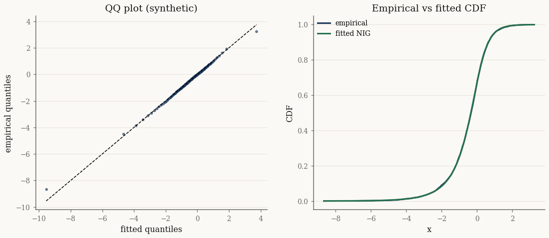
The KS statistic against a large sample from the fit is small, as expected when the model is correct:

ks = stats.ks_2samp(x_syn, np.asarray(fit.rvs(50_000, seed=1)))
print(f"KS statistic = {ks.statistic:.4f},  p-value = {ks.pvalue:.3f}")

KS statistic = 0.0077,  p-value = 0.978

Real data: heavy tails in equity returns

Now a real series — Apple daily log returns — where the Gaussian famously fails. We fit a NIG and compare it against a normal of the same mean and variance:

data_path = Path("../../../data/sp500_returns.csv").resolve()
returns = pd.read_csv(data_path, index_col="Date", parse_dates=True)
x = np.asarray(returns["AAPL"].dropna().values, dtype=np.float64)
print(f"AAPL: {len(x)} daily returns,  excess kurtosis = {stats.kurtosis(x):.2f}")

fit_real = fit_univariate_nig(x, max_iter=120, tol=1e-4, e_step_backend="cpu")

AAPL: 2552 daily returns,  excess kurtosis = 6.67

fig, (aq, ax_t) = plt.subplots(1, 2, figsize=(12, 4.6))

# QQ: NIG vs Normal
theo_nig, emp = qq_points(x, fit_real)
mu_g, sd_g = x.mean(), x.std()
probs = (np.arange(1, len(x) + 1) - 0.5) / len(x)
idx = np.linspace(0, len(x) - 1, 150).astype(int)
theo_norm = stats.norm.ppf(probs[idx], loc=mu_g, scale=sd_g)

lim = [emp.min(), emp.max()]
aq.scatter(theo_norm, emp, s=8, alpha=0.5, label="Normal")
aq.scatter(theo_nig, emp, s=8, alpha=0.6, label="NIG")
aq.plot(lim, lim, "k--", lw=1)
aq.set_xlabel("model quantiles"); aq.set_ylabel("empirical quantiles")
aq.set_title("QQ plot: AAPL returns"); aq.legend()

# Tail of the density (log scale)
grid = jnp.linspace(float(x.min()), float(x.max()), 400)
ax_t.hist(x, bins=120, density=True, alpha=0.35, color="0.6", label="returns")
ax_t.plot(np.asarray(grid), np.asarray(jax.vmap(fit_real.pdf)(grid)), label="NIG")
ax_t.plot(np.asarray(grid), stats.norm.pdf(np.asarray(grid), mu_g, sd_g),
          "k--", lw=1.2, label="Normal")
ax_t.set_yscale("log"); ax_t.set_ylim(1e-1, None)
ax_t.set_xlabel("daily log return"); ax_t.set_ylabel("density (log scale)")
ax_t.set_title("Density fit"); ax_t.legend()
plt.show()

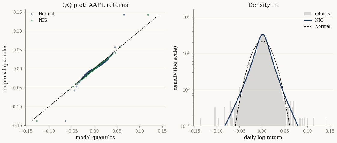
The Gaussian QQ points bend away from the diagonal in both tails — it under-predicts extreme moves. The NIG points hug the diagonal, and the log-density panel shows it capturing the heavy tails the normal misses. The KS test confirms it numerically:

ks_nig = stats.ks_2samp(x, np.asarray(fit_real.rvs(50_000, seed=2)))
ks_norm = stats.kstest(x, "norm", args=(mu_g, sd_g))
print(f"NIG    : KS = {ks_nig.statistic:.4f},  p = {ks_nig.pvalue:.3g}")
print(f"Normal : KS = {ks_norm.statistic:.4f},  p = {ks_norm.pvalue:.3g}")

NIG    : KS = 0.0110,  p = 0.928
Normal : KS = 0.0824,  p = 1.55e-15

Takeaways

• Fit a 1-D marginal on (n, 1) data, then convert to a Univariate* object for cdf / ppf.

• QQ plots and CDF overlays are the workhorse visual diagnostics; KS (via ks_2samp against a large model sample) gives a numerical summary.

• On real equity returns the NIG tracks the heavy tails that the Gaussian misses.

This concludes the statistics section. The A heavy-tailed index series tutorial puts these tools to work on real market data.