Portfolio CVaR and its derivatives#

The payoff of modelling returns with a normal variance-mean mixture is that tail risk becomes tractable. Conditional on the latent \(Y\), a portfolio is Gaussian, so the Conditional Value-at-Risk \(\operatorname{CVaR}_\alpha\) — and its gradient and Hessian in the portfolio weights — can be computed by a fast conditional Monte Carlo over \(Y\) alone. This tutorial fits a mixture, computes CVaR, verifies the analytic derivatives, and takes a few gradient steps to reduce risk.

import jax
jax.config.update("jax_enable_x64", True)
import jax.numpy as jnp
import numpy as np
import pandas as pd
from pathlib import Path

from normix import NormalInverseGaussian, UnivariateNormalInverseGaussian
from normix.finance import project_portfolio, CVaR
from normix.utils.plotting import set_theme

set_theme()
np.set_printoptions(precision=5, suppress=True)

A fitted mixture and a portfolio#

basket = ["AAPL", "MSFT", "JPM", "XOM"]
data_path = Path("../../../data/sp500_returns.csv").resolve()
R = pd.read_csv(data_path, index_col="Date", parse_dates=True)[basket].dropna()
X = jnp.asarray(R.values, dtype=jnp.float64)

model = NormalInverseGaussian.default_init(X).fit(
    X, max_iter=120, tol=1e-4, e_step_backend="cpu").model

w = jnp.array([0.4, 0.3, 0.2, 0.1])
proj = project_portfolio(model, w)         # 1-D return distribution of wᵀX
alpha = 0.05
cvar = CVaR(alpha)
print(f"portfolio mean {float(proj.mean()):+.5f}, std {float(proj.std()):.5f}")

portfolio mean +0.00082, std 0.01318

VaR, CVaR, and conditional Monte Carlo#

VaR is a deterministic quantile via the projected ppf. CVaR uses a conditional Monte Carlo over the subordinator draws \(Y\) — far lower variance than sampling returns directly:

Y = proj.subordinator.rvs(100_000, seed=0)
var_a = float(cvar.var(proj))
cvar_a = float(cvar.value(proj, Y))
print(f"VaR_{1-alpha:.0%}  = {var_a:.5f}")
print(f"CVaR_{1-alpha:.0%} = {cvar_a:.5f}")

VaR_95%  = 0.02048
CVaR_95% = 0.03094

We validate against a brute-force quantile estimate from one million return draws — agreement confirms the conditional-MC estimator:

draws = jnp.sort(proj.rvs(1_000_000, seed=1))
k = int(alpha * draws.shape[0])
cvar_brute = float(-draws[:k].mean())
print(f"conditional-MC CVaR : {cvar_a:.5f}")
print(f"brute-force MC CVaR : {cvar_brute:.5f}")

conditional-MC CVaR : 0.03094
brute-force MC CVaR : 0.03095

Derivatives in the scalar parametrization#

CVaR differentiates the risk analytically in the projected parameters \((\tilde\mu, \tilde\gamma, \tilde\sigma)\). We check the gradient against a central finite difference using common random numbers (the same \(Y\)):

sub = proj.subordinator
mt, gt, st = float(proj._mu_scalar), float(proj._gamma_scalar), float(proj._sigma_scalar)

def rebuild(m, g, s):
    return UnivariateNormalInverseGaussian.from_classical(
        mu=m, gamma=g, sigma=s ** 2, mu_ig=float(sub.mu), lam=float(sub.lam))

g_analytic = np.asarray(cvar.gradient_scalar(proj, Y))
eps = 1e-5
g_fd = []
for i, base in enumerate((mt, gt, st)):
    hi, lo = [mt, gt, st], [mt, gt, st]
    hi[i] += eps; lo[i] -= eps
    g_fd.append((float(cvar.value(rebuild(*hi), Y)) - float(cvar.value(rebuild(*lo), Y))) / (2 * eps))

print("∂CVaR/∂(μ̃, γ̃, σ̃) analytic:", g_analytic)
print("∂CVaR/∂(μ̃, γ̃, σ̃) FD      :", np.array(g_fd))

∂CVaR/∂(μ̃, γ̃, σ̃) analytic: [-1.      -2.05454  2.10208]
∂CVaR/∂(μ̃, γ̃, σ̃) FD      : [-1.      -2.05454  2.10208]

The leading \(-1\) is exact: shifting the mean shifts CVaR one-for-one.

Derivatives in weight space#

For optimization we need the gradient in the weights \(w\) directly. gradient_w and hessian_w apply the chain rule through the projection; we verify the gradient against a finite difference of value_w:

gw_analytic = np.asarray(cvar.gradient_w(model, w, Y))
gw_fd = []
for i in range(len(w)):
    hi, lo = w.at[i].add(eps), w.at[i].add(-eps)
    gw_fd.append((float(cvar.value_w(model, hi, Y)) - float(cvar.value_w(model, lo, Y))) / (2 * eps))

print("∇_w CVaR analytic:", gw_analytic)
print("∇_w CVaR FD      :", np.array(gw_fd))
print("Hessian_w shape  :", np.asarray(cvar.hessian_w(model, w, Y)).shape)

∇_w CVaR analytic: [0.03715 0.03175 0.02403 0.0175 ]
∇_w CVaR FD      : [0.03715 0.03175 0.02403 0.0175 ]
Hessian_w shape  : (4, 4)

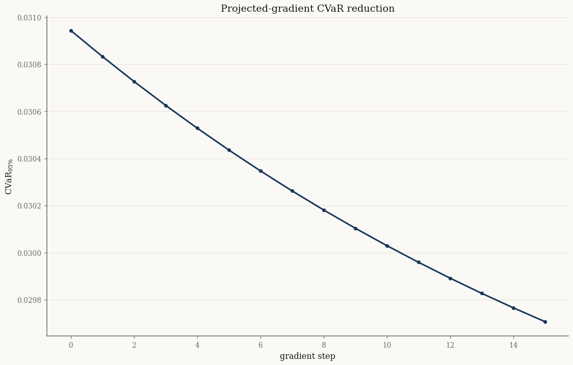
A few risk-reducing steps#

Projected gradient descent on the weights (keeping \(\sum_i w_i = 1\)) reduces the portfolio CVaR. We hold \(Y\) fixed across steps for a clean comparison:

w_opt = w
path = [float(cvar.value_w(model, w_opt, Y))]
lr = 0.5
for _ in range(15):
    g = cvar.gradient_w(model, w_opt, Y)
    g = g - g.mean()                       # project onto the simplex tangent (Σ Δw = 0)
    w_opt = w_opt - lr * g
    path.append(float(cvar.value_w(model, w_opt, Y)))

print(f"start weights : {np.asarray(w)}")
print(f"final weights : {np.asarray(w_opt)}  (sum {float(w_opt.sum()):.4f})")
print(f"CVaR {path[0]:.5f} → {path[-1]:.5f}")

start weights : [0.4 0.3 0.2 0.1]
final weights : [0.33703 0.27551 0.22263 0.16484]  (sum 1.0000)
CVaR 0.03094 → 0.02971

import matplotlib.pyplot as plt

fig, ax = plt.subplots()
ax.plot(path, "o-")
ax.set_xlabel("gradient step"); ax.set_ylabel(r"$\mathrm{CVaR}_{95\%}$")
ax.set_title("Projected-gradient CVaR reduction")
plt.show()

../../_images/96fc26a0a82a6cc5066fcd7f70998125c825c5a10762d9f246a97cbfb29965c3.png

The weight gradient lets you plug normix’s tail risk straight into any constrained optimizer; the analytic Hessian enables second-order methods.

Takeaways#

A fitted mixture yields portfolio VaR and CVaR through a low-variance conditional Monte Carlo over the subordinator \(Y\) — validated against brute-force sampling.
CVaR provides analytic gradients/Hessians in both \((\tilde\mu, \tilde\gamma, \tilde\sigma)\) and the weights \(w\), matching finite differences to machine precision.
Those weight-space derivatives drive gradient-based CVaR optimization.

This concludes the finance section. See the Finance overview for how these pieces fit together.

Portfolio CVaR and its derivatives

Contents