Gamma

The Gamma distribution on \((0, \infty)\) with shape \(\alpha > 0\) and rate \(\beta > 0\):

\[ f(x \mid \alpha, \beta) = \frac{\beta^\alpha}{\Gamma(\alpha)}\, x^{\alpha-1} e^{-\beta x}, \qquad x > 0. \]

It is the \(b \to 0\) limit of the GIG and, as a subordinator, gives rise to the VarianceGamma mixture. All moments and the MLE are closed-form.

Density gallery

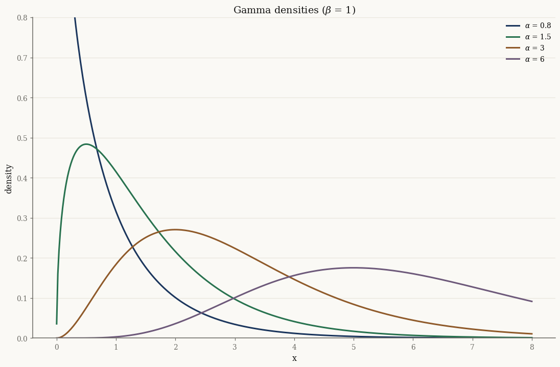
The shape \(\alpha\) interpolates from a monotone-decreasing density (\(\alpha < 1\), diverging at the origin) through the exponential (\(\alpha = 1\)) to an increasingly symmetric bell (\(\alpha \gg 1\)).

Show code cell source

Hide code cell source

import jax
jax.config.update("jax_enable_x64", True)
import jax.numpy as jnp
import numpy as np
import matplotlib.pyplot as plt

from normix import Gamma
from normix.utils.plotting import set_theme

set_theme()
np.set_printoptions(precision=5, suppress=True)

x = jnp.linspace(1e-3, 8.0, 400)
fig, ax = plt.subplots()
for alpha in [0.8, 1.5, 3.0, 6.0]:
    g = Gamma(alpha=jnp.array(alpha), beta=jnp.array(1.0))
    ax.plot(np.asarray(x), np.asarray(jax.vmap(g.pdf)(x)), label=rf"$\alpha$ = {alpha:g}")
ax.set_ylim(0, 0.8)
ax.set_xlabel("x"); ax.set_ylabel("density")
ax.set_title(r"Gamma densities ($\beta$ = 1)")
ax.legend()
plt.show()

Parametrizations

Stored attributes: alpha, beta. Exponential family with sufficient statistic \(t(x) = [\log x,\; x]\):

Parametrization	Value
Classical	shape \(\alpha > 0\), rate \(\beta > 0\)
Natural \(\theta\)	\([\,\alpha - 1,\; -\beta\,]\)
Expectation \(\eta = \nabla\psi\)	\([\,\psi(\alpha) - \log\beta,\; \alpha/\beta\,] = (\mathbb{E}[\log X],\; \mathbb{E}[X])\)

where \(\psi\) is the digamma function. The \(\eta \mapsto \theta\) inversion is a scalar Newton solve on the digamma equation (closed-form).

Quick usage

gamma = Gamma(alpha=jnp.array(2.5), beta=jnp.array(1.5))

print("mean/var/std:", float(gamma.mean()), float(gamma.var()), float(gamma.std()))
print("cdf(2.0):    ", float(gamma.cdf(jnp.array(2.0))))
print("5% quantile: ", float(gamma.ppf(jnp.array(0.05))))

samples = gamma.rvs(10_000, seed=0)
fitted = Gamma.fit_mle(samples)            # moment-matching MLE
print("fit (a,b):   ", float(fitted.alpha), float(fitted.beta))

mean/var/std: 1.6666666666666667 1.1111111111111112 1.0540925533894598
cdf(2.0):     0.6937810815867218
5% quantile:  0.3818254086872564
fit (a,b):    2.501355473646757 1.5000528913010398

See also

• API: Gamma

• Theory: The Generalized Inverse Gaussian Distribution — Gamma as a limit of the GIG family

• Tutorial: Univariate positive distributions