Random sampling#

Every normix distribution can generate samples through a uniform rvs(n, seed) interface. Under the hood the methods range from textbook inverse-CDF sampling to the Devroye ratio-of-uniforms rejection sampler for the GIG. This tutorial shows the interface, validates the samplers against references, and explains the GIG sampling options.

import jax
jax.config.update("jax_enable_x64", True)
import jax.numpy as jnp
import numpy as np
from scipy import stats

from normix import (
    Gamma, InverseGaussian, GIG, MultivariateNormal,
    NormalInverseGaussian, GeneralizedHyperbolic,
)
from normix.utils.plotting import set_theme

set_theme()

The `rvs` interface#

rvs(n, seed) returns an array of n draws and is fully reproducible: the same integer seed always yields identical samples.

g = Gamma(alpha=jnp.array(2.5), beta=jnp.array(1.5))
s1 = g.rvs(5, seed=0)
s2 = g.rvs(5, seed=0)
print("reproducible:", bool(jnp.array_equal(s1, s2)))
print("samples:", np.asarray(s1))

reproducible: True
samples: [1.20325347 1.02570646 2.96166115 0.25375372 1.54408211]

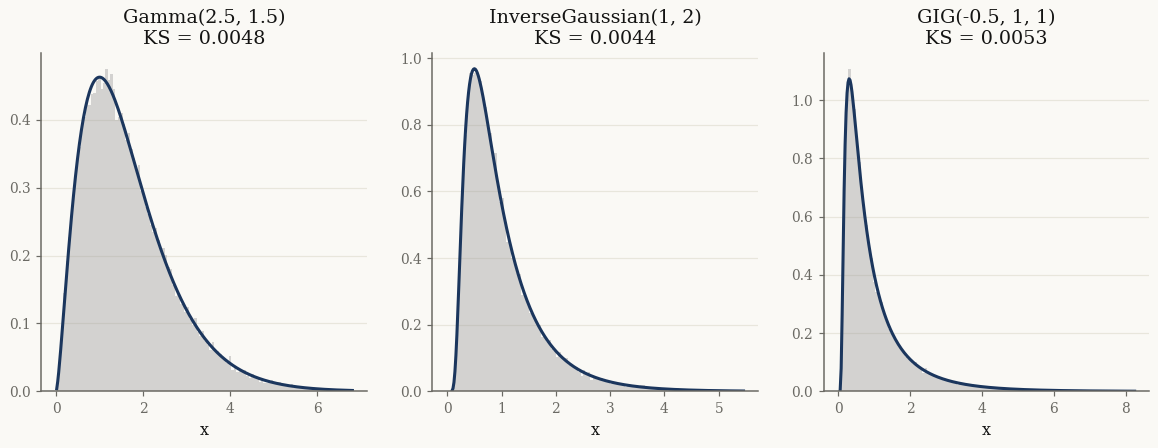
Validating univariate samplers#

We draw from three univariate distributions and overlay the analytic density. The Kolmogorov–Smirnov statistic against the true CDF stays small:

import matplotlib.pyplot as plt

dists = {
    "Gamma(2.5, 1.5)": Gamma(alpha=jnp.array(2.5), beta=jnp.array(1.5)),
    "InverseGaussian(1, 2)": InverseGaussian(mu=jnp.array(1.0), lam=jnp.array(2.0)),
    "GIG(-0.5, 1, 1)": GIG(p=jnp.array(-0.5), a=jnp.array(1.0), b=jnp.array(1.0)),
}

fig, axes = plt.subplots(1, 3, figsize=(13, 4))
for ax, (name, d) in zip(axes, dists.items()):
    x = np.asarray(d.rvs(50_000, seed=1))
    ks = stats.kstest(x, lambda q: np.asarray(jax.vmap(d.cdf)(jnp.asarray(q)))).statistic
    grid = jnp.linspace(max(1e-3, x.min()), np.quantile(x, 0.999), 300)
    ax.hist(x, bins=120, density=True, range=(0, float(grid.max())),
            alpha=0.4, color="0.6")
    ax.plot(np.asarray(grid), np.asarray(jax.vmap(d.pdf)(grid)), lw=2)
    ax.set_title(f"{name}\nKS = {ks:.4f}")
    ax.set_xlabel("x")
plt.show()

../../_images/9063d3b0921705ba6ac65b7c0dc5895aa75879cd935e981133d94a272fd46d8c.png

GIG sampling methods#

The GIG is the only distribution with a genuine sampling choice. rvs accepts a method:

"devroye" (default) — Devroye’s ratio-of-uniforms rejection sampler; exact and the most robust across parameter regimes.
"pinv" — Polynomial inverse-CDF (numerical inversion); fast for repeated draws from a fixed parameter set.
"scipy" — delegates to scipy.stats.geninvgauss (reference / CPU only).

All three target the same distribution; their empirical moments agree:

gig = GIG(p=jnp.array(1.2), a=jnp.array(2.0), b=jnp.array(1.5))
print(f"{'method':>8s}   {'mean':>8s}  {'var':>8s}")
print(f"{'analytic':>8s}   {float(gig.mean()):8.4f}  {float(gig.var()):8.4f}")
for method in ["devroye", "pinv", "scipy"]:
    x = gig.rvs(100_000, seed=7, method=method)
    print(f"{method:>8s}   {float(x.mean()):8.4f}  {float(x.var()):8.4f}")

  method       mean       var
analytic     1.8273    1.4310
 devroye     1.8224    1.4140
    pinv     1.8281    1.4470
   scipy     1.8333    1.4347

Multivariate sampling#

For multivariate distributions rvs(n, seed) returns an (n, d) array. The MultivariateNormal draws Gaussians:

mvn = MultivariateNormal.from_classical(
    mu=jnp.array([0.0, 1.0]),
    sigma=jnp.array([[1.0, 0.6], [0.6, 2.0]]))
Xn = mvn.rvs(20_000, seed=0)
print("shape:", Xn.shape)
print("empirical mean:", np.asarray(Xn.mean(axis=0)))
print("empirical cov:\n", np.cov(np.asarray(Xn), rowvar=False))

shape: (20000, 2)
empirical mean: [-0.01195784  0.98016401]
empirical cov:
 [[1.0095161  0.59840201]
 [0.59840201 1.97882088]]

Marginal vs joint sampling#

A mixture distribution exposes two samplers. The marginal rvs returns just the observations \(X\); the joint rvs (on .joint) also returns the latent subordinator draws \(Y\) used to generate them:

nig = NormalInverseGaussian.from_classical(
    mu=jnp.array([0.0, 0.0]),
    gamma=jnp.array([0.3, -0.2]),
    sigma=jnp.array([[1.0, 0.4], [0.4, 1.0]]),
    mu_ig=1.0, lam=1.5)

X = nig.rvs(10_000, seed=3)             # marginal: X only, shape (n, d)
Xj, Y = nig.joint.rvs(10_000, seed=3)   # joint: (X, Y)
print("marginal X:", X.shape)
print("joint    X:", Xj.shape, " Y:", Y.shape)
print("same draws:", bool(jnp.allclose(X, Xj)))
print("E[Y] =", float(Y.mean()))

marginal X: (10000, 2)
joint    X: (10000, 2)  Y: (10000,)
same draws: True
E[Y] = 0.9996950920607215

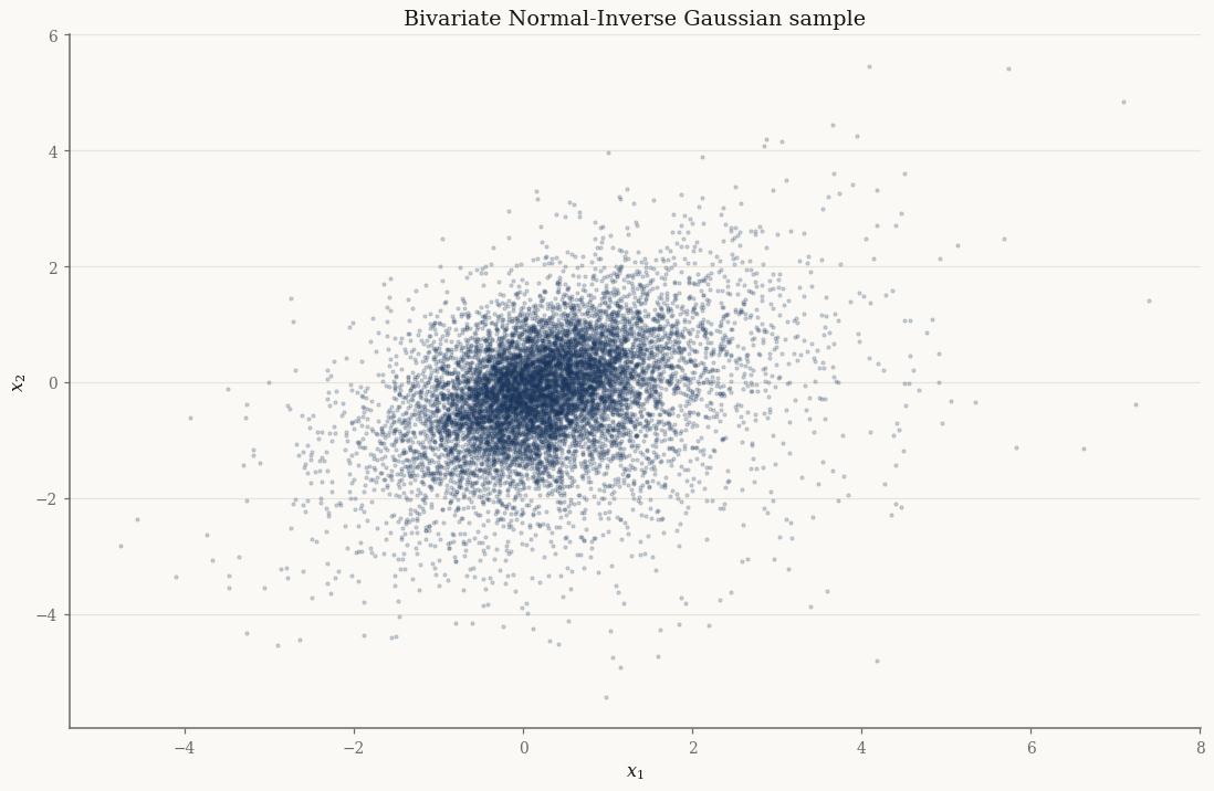
Having \(Y\) in hand is what makes the EM E-step possible: the conditional moments \(\mathbb{E}[\,\cdot \mid X]\) are computed from this latent structure.

fig, ax = plt.subplots()
ax.scatter(np.asarray(X[:, 0]), np.asarray(X[:, 1]), s=4, alpha=0.2)
ax.set_xlabel("$x_1$"); ax.set_ylabel("$x_2$")
ax.set_title("Bivariate Normal-Inverse Gaussian sample")
plt.show()

../../_images/ef3f8edc41c7ae3d4732beafba32b7ab71cde7276efc11d81b3f70bb8567ee32.png

Takeaways#

rvs(n, seed) is the uniform, reproducible sampling interface; multivariate draws come back as (n, d).
The GIG offers method ∈ {"devroye", "pinv", "scipy"}, all sampling the same law — "devroye" is the robust default.
Mixture marginals sample \(X\); their .joint samples \((X, Y)\) including the latent subordinator.

Next, the Univariate positive distributions tour exercises every constructor and method on the concrete distribution classes.

Random sampling

Contents