Transaction costs and local-quadratic rebalancing#
The mean-risk reduction of Mean-risk optimization and the efficient surface collapses portfolio choice to two coordinates \((\tilde\mu, \tilde\gamma)\). An \(\ell_1\) turnover penalty breaks that reduction: \(\|w - w_0\|_1\) is not a function of the reduced coordinates alone. When transaction costs keep the solution near the current portfolio \(w_0\), a second-order Taylor expansion of the coherent risk \(r\) recovers a quadratic program in buy/sell variables. This tutorial walks through that construction on the same Dow basket used in the mean-risk page.
Formal derivation: Portfolio Optimization with Transaction Costs.
This page is intentionally separate from
Mean-risk optimization and the efficient surface: that tutorial is about the frictionless
dimension reduction; here the turnover term breaks that reduction and the
API is a different object (TransactionCostProblem).
import jax
jax.config.update("jax_enable_x64", True)
import jax.numpy as jnp
import numpy as np
import pandas as pd
from pathlib import Path

from normix import GeneralizedHyperbolic
from normix.finance import CVaR, MeanRiskProblem, TransactionCostProblem
from normix.utils.plotting import set_theme, COLORS

set_theme()
np.set_printoptions(precision=5, suppress=True)
Fit once, rebalance often#
basket = ["AAPL", "MSFT", "JPM", "XOM", "JNJ", "PG", "WMT", "CAT"]
data_path = Path("../../../data/sp500_returns.csv").resolve()
R = pd.read_csv(data_path, index_col="Date", parse_dates=True)[basket].dropna()
X = jnp.asarray(R.values, dtype=jnp.float64)

model = (GeneralizedHyperbolic.default_init(X)
         .fit(X, max_iter=100, tol=1e-4, e_step_backend="cpu").model
         .regularize_a_eq_b())
cvar = CVaR(0.05)
Y = model.joint.subordinator().rvs(15_000, seed=0)
print(f"mean log-likelihood {float(model.marginal_log_likelihood(X)):.4f}")
mean log-likelihood 24.1906
Take the minimum-CVaR frontier portfolio as the current holding \(w_0\) — a manager who already solved the frictionless problem and now faces a cost of trading.
prob = MeanRiskProblem(model, cvar)
mv_mu, mv_gamma = prob.min_variance_point()
mv_ret = float(prob.expected_return(mv_mu, mv_gamma))
targets = jnp.linspace(mv_ret, mv_ret + 4e-4, 25)
ga = float(mv_gamma)
span = 1.5 * max(float(np.asarray(model.gamma).max()
                      - np.asarray(model.gamma).min()), 4e-4)
frontier = prob.efficient_frontier(
    targets, Y, gamma_bounds=(ga - span, ga + span), n_iter=40)
k = int(np.argmin(np.asarray(frontier.risk)))
w0 = frontier.weights[k]
print(f"anchor return {float(frontier.expected_return[k]):.3e}  "
      f"CVaR {float(frontier.risk[k]):.4f}")
pd.Series(np.asarray(w0), index=basket).round(3)
anchor return 5.538e-04 CVaR 0.0194
AAPL    0.011
MSFT    0.039
JPM     0.058
XOM     0.106
JNJ     0.309
PG      0.237
WMT     0.233
CAT     0.008
dtype: float64
Local quadratic program#
TransactionCostProblem reuses the same CVaR object — only its weight-space
gradient and Hessian at \(w_0\) enter the QP. The objective is
approximated by replacing \(r\) with its Taylor model at \(w_0\) and introducing buy/sell variables \(v = (v^+; v^-)\).
tc = TransactionCostProblem(model, cvar, c1=5.0, c2=5e-2)
A = -jnp.eye(len(basket), dtype=jnp.float64)   # long-only: -w ≤ 0
b = jnp.zeros(len(basket), dtype=jnp.float64)
result = tc.solve(w0, Y, A=A, b=b)

print(f"improved over hold?  {bool(result.improved)}")
print(f"turnover ‖Δw‖₁      {float(result.turnover):.4f}")
print(f"approx obj  hold → * {float(result.hold_objective):.6e} → "
      f"{float(result.approx_objective):.6e}")
print(f"exact  obj  hold → * {float(tc.true_objective_at(w0, w0, Y)):.6e} → "
      f"{float(tc.true_objective_at(result.weights, w0, Y)):.6e}")
improved over hold?  False
turnover ‖Δw‖₁      0.0000
approx obj  hold → * -9.664417e-02 → -9.664417e-02
exact  obj  hold → * -9.664417e-02 → -9.664417e-02
The matrices themselves are available for an external QP solver if needed:
qp = result.qp
print(f"m̃ shape {qp.m_tilde.shape},  H̃ shape {qp.H_tilde.shape}")
print(f"budget residual ẽᵀv = {float(qp.e_tilde @ result.v):.2e}")
m̃ shape (16,),  H̃ shape (16, 16)
budget residual ẽᵀv = 0.00e+00
How costs reshape the trade#
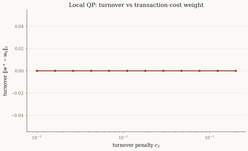
Sweeping \(c_2\) shows the continuum from frictionless rebalancing to a pure hold.
import matplotlib.pyplot as plt

c2_grid = np.geomspace(1e-3, 2e-1, 12)
rows = []
for c2 in c2_grid:
    r = TransactionCostProblem(model, cvar, c1=5.0, c2=float(c2)).solve(
        w0, Y, A=A, b=b)
    rows.append({
        "c2": c2,
        "turnover": float(r.turnover),
        "approx_gain": float(r.approx_objective - r.hold_objective),
        "exact_gain": float(
            tc.true_objective_at(r.weights, w0, Y)
            - tc.true_objective_at(w0, w0, Y)
        ) if bool(r.improved) else 0.0,
    })
sweep = pd.DataFrame(rows)

fig, ax = plt.subplots(figsize=(8.5, 4.8))
ax.plot(sweep["c2"], sweep["turnover"], "o-", color=COLORS["brick"], lw=2)
ax.set_xscale("log")
ax.set_xlabel(r"turnover penalty $c_2$")
ax.set_ylabel(r"turnover $\|w^\star - w_0\|_1$")
ax.set_title("Local QP: turnover vs transaction-cost weight")
plt.show()
sweep.round(5)
| c2 | turnover | approx_gain | exact_gain | |
|---|---|---|---|---|
| 0 | 0.00100 | 0.0 | 0.0 | 0.0 |
| 1 | 0.00162 | 0.0 | 0.0 | 0.0 |
| 2 | 0.00262 | 0.0 | 0.0 | 0.0 |
| 3 | 0.00424 | 0.0 | 0.0 | 0.0 |
| 4 | 0.00687 | 0.0 | 0.0 | 0.0 |
| 5 | 0.01112 | 0.0 | 0.0 | 0.0 |
| 6 | 0.01799 | 0.0 | 0.0 | 0.0 |
| 7 | 0.02913 | 0.0 | 0.0 | 0.0 |
| 8 | 0.04715 | 0.0 | 0.0 | 0.0 |
| 9 | 0.07632 | 0.0 | 0.0 | 0.0 |
| 10 | 0.12355 | 0.0 | 0.0 | 0.0 |
| 11 | 0.20000 | 0.0 | 0.0 | 0.0 |
At large \(c_2\) the solver correctly returns the hold (\(w^\star = w_0\)). At small \(c_2\) the quadratic model can recommend a large move — outside the regime where the Taylor expansion is trustworthy — so in practice one verifies that the exact Monte Carlo objective also improves, exactly as the theory note warns.
cmp = pd.DataFrame(
    {"w0": np.asarray(w0), "w*": np.asarray(result.weights)},
    index=basket,
)
cmp["Δ"] = cmp["w*"] - cmp["w0"]
cmp.round(3)
| w0 | w* | Δ | |
|---|---|---|---|
| AAPL | 0.011 | 0.011 | 0.0 |
| MSFT | 0.039 | 0.039 | 0.0 |
| JPM | 0.058 | 0.058 | 0.0 |
| XOM | 0.106 | 0.106 | 0.0 |
| JNJ | 0.309 | 0.309 | 0.0 |
| PG | 0.237 | 0.237 | 0.0 |
| WMT | 0.233 | 0.233 | 0.0 |
| CAT | 0.008 | 0.008 | 0.0 |
Takeaways#
Transaction costs live in an optimization layer, not inside the risk measure: the same
CVaRobject feeds both the efficient surface and the local QP.TransactionCostProblem.build_qpexposes the theory matrices \((\tilde m, \tilde H, \tilde e, \tilde A, \tilde b)\);.solveruns a SciPy SLSQP default without adding a QP dependency.Always check
improved(and ideally the exact objective): if the approximate gain is non-positive, hold \(w_0\).
See Portfolio Optimization with Transaction Costs for the QP derivation and Mean-risk optimization and the efficient surface for the frictionless surface this rebalancing starts from.