Univariate positive distributions

Gamma, InverseGamma, and InverseGaussian are the building blocks of the GH family — they are the subordinators that drive the mixtures. They are also the distributions with the cleanest exponential-family structure: their moments and maximum-likelihood estimates are available in closed form, so the log-partition triad uses analytical gradients (digamma / trigamma) rather than autodiff.

import jax
jax.config.update("jax_enable_x64", True)
import jax.numpy as jnp
import numpy as np

from normix import Gamma, InverseGamma, InverseGaussian
from normix.utils.plotting import set_theme

set_theme()
np.set_printoptions(precision=5, suppress=True)

Construction and moments

Each distribution is built directly from its classical parameters and reports its first two moments:

dists = {
    "Gamma(α=2.5, β=1.5)": Gamma(alpha=jnp.array(2.5), beta=jnp.array(1.5)),
    "InverseGamma(α=3, β=2)": InverseGamma(alpha=jnp.array(3.0), beta=jnp.array(2.0)),
    "InverseGaussian(μ=1, λ=3)": InverseGaussian(mu=jnp.array(1.0), lam=jnp.array(3.0)),
}
print(f"{'distribution':28s} {'mean':>8s} {'var':>8s} {'std':>8s}")
for name, d in dists.items():
    print(f"{name:28s} {float(d.mean()):8.4f} {float(d.var()):8.4f} {float(d.std()):8.4f}")

distribution                     mean      var      std
Gamma(α=2.5, β=1.5)            1.6667   1.1111   1.0541
InverseGamma(α=3, β=2)         1.0000   1.0000   1.0000
InverseGaussian(μ=1, λ=3)      1.0000   0.3333   0.5774

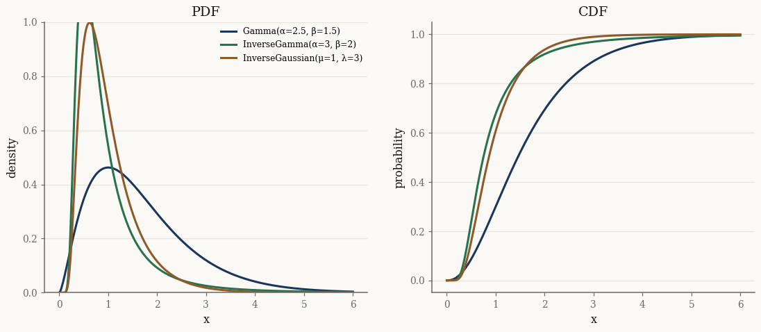
Density, CDF, and quantiles

All three provide pdf, cdf, and the quantile function ppf. cdf and ppf are mutual inverses:

d = dists["Gamma(α=2.5, β=1.5)"]
q = jnp.array([0.1, 0.5, 0.9])
x_q = jax.vmap(d.ppf)(q)
back = jax.vmap(d.cdf)(x_q)
print("quantiles x_q :", np.asarray(x_q))
print("cdf(ppf(q))   :", np.asarray(back))

quantiles x_q : [0.53677 1.45049 3.07879]
cdf(ppf(q))   : [0.1 0.5 0.9]

import matplotlib.pyplot as plt

x = jnp.linspace(1e-3, 6.0, 400)
fig, (axp, axc) = plt.subplots(1, 2, figsize=(12, 4.6))
for name, d in dists.items():
    axp.plot(np.asarray(x), np.asarray(jax.vmap(d.pdf)(x)), label=name)
    axc.plot(np.asarray(x), np.asarray(jax.vmap(d.cdf)(x)), label=name)
axp.set_title("PDF"); axp.set_xlabel("x"); axp.set_ylabel("density")
axc.set_title("CDF"); axc.set_xlabel("x"); axc.set_ylabel("probability")
axp.set_ylim(0, 1.0); axp.legend(fontsize=8)
plt.show()

Three parametrizations

As exponential families they expose natural (\(\theta\)) and expectation (\(\eta\)) parameters. For Gamma, \(\eta = (\mathbb{E}[\log X],\, \mathbb{E}[X])\), and the round-trip back to classical parameters is exact:

g = dists["Gamma(α=2.5, β=1.5)"]
theta = g.natural_params()
eta = g.expectation_params()
print("theta =", np.asarray(theta))
print("eta   = (E[log X], E[X]) =", np.asarray(eta))

g_back = Gamma.from_expectation(eta)
print("recovered (alpha, beta):", float(g_back.alpha), float(g_back.beta))

theta = [ 1.5 -1.5]
eta   = (E[log X], E[X]) = [0.29769 1.66667]
recovered (alpha, beta): 2.500000000000004 1.5000000000000022

Closed-form maximum likelihood

Because the MLE matches moments, fit_mle recovers parameters from samples in a single call. We draw from each distribution and refit:

for name, d in dists.items():
    x = d.rvs(50_000, seed=0)
    if isinstance(d, Gamma):
        fitted = Gamma.fit_mle(x)
        true_p, fit_p = (d.alpha, d.beta), (fitted.alpha, fitted.beta)
    elif isinstance(d, InverseGamma):
        fitted = InverseGamma.fit_mle(x)
        true_p, fit_p = (d.alpha, d.beta), (fitted.alpha, fitted.beta)
    else:
        fitted = InverseGaussian.fit_mle(x)
        true_p, fit_p = (d.mu, d.lam), (fitted.mu, fitted.lam)
    true_p = tuple(round(float(v), 3) for v in true_p)
    fit_p = tuple(round(float(v), 3) for v in fit_p)
    print(f"{name:28s} true={true_p}  mle={fit_p}")

Gamma(α=2.5, β=1.5)          true=(2.5, 1.5)  mle=(2.461, 1.476)
InverseGamma(α=3, β=2)       true=(3.0, 2.0)  mle=(2.951, 1.968)
InverseGaussian(μ=1, λ=3)    true=(1.0, 3.0)  mle=(1.0, 2.98)

The analytical triad means none of this routes through a generic optimizer: the gradient of the log-partition is digamma, its Hessian is trigamma, and from_expectation inverts them directly.

Takeaways

• Gamma, InverseGamma, InverseGaussian provide pdf, cdf, ppf, mean/var/std, and rvs.

• They carry analytical log-partition gradients, so moments and fit_mle are closed-form and fast.

• These three are exactly the subordinators behind VG, NInvG, and NIG.

Next: The Generalized Inverse Gaussian covers the GIG, where the log-partition involves Bessel functions and from_expectation needs a multi-start solver.