A multivariate stock basket#

Real returns are not only heavy-tailed but jointly so: extreme days hit assets together. A normal variance-mean mixture captures this with a single shared latent factor \(Y\) — a market-wide “volatility” that inflates every asset’s variance on the same days. Here we fit a full-covariance mixture to a small basket and read off that latent factor.

import jax
jax.config.update("jax_enable_x64", True)
import jax.numpy as jnp
import numpy as np
import pandas as pd
from pathlib import Path

from normix import NormalInverseGaussian
from normix.finance import project_portfolio
from normix.fitting.em import BatchEMFitter
from normix.utils.plotting import set_theme

set_theme()
np.set_printoptions(precision=4, suppress=True)

Data: a five-stock basket#

basket = ["AAPL", "MSFT", "JPM", "XOM", "PG"]
data_path = Path("../../../data/sp500_returns.csv").resolve()
panel = pd.read_csv(data_path, index_col="Date", parse_dates=True)[basket].dropna()

dates = panel.index
R = panel.values.astype(np.float64)
n_train = len(R) // 2
X_train = jnp.asarray(R[:n_train])
X_test = jnp.asarray(R[n_train:])
print(f"{R.shape[0]} days × {R.shape[1]} stocks; train {n_train}, test {R.shape[0]-n_train}")

2552 days × 5 stocks; train 1276, test 1276

Fitting with EM on real data#

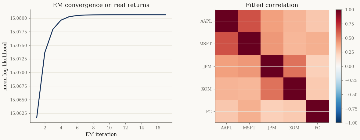
We fit a full-\(\Sigma\) NIG and watch the EM log-likelihood ascend on genuine market data:

init = NormalInverseGaussian.default_init(X_train)
fitter = BatchEMFitter(max_iter=150, tol=1e-4, verbose=1,
                       e_step_backend="cpu", m_step_backend="cpu")
result = fitter.fit(init, X_train)
model = result.model
print(f"converged {result.converged} in {result.n_iter} iters ({result.elapsed_time:.1f}s)")
print(f"test mean log-lik: {float(model.marginal_log_likelihood(X_test)):.4f}")

============================================================
  EM Fitting: NormalInverseGaussian
============================================================
  Algorithm    : EM
  Loop         : Python loop
  E-step       : cpu
  M-step       : cpu / newton
  Regularize   : none
  Tolerance    : 1.0e-04
  Max iters    : 150
  Converged after 17 iterations (7.46s), final LL=15.080614
converged True in 17 iters (7.5s)
test mean log-lik: 14.3791

import matplotlib.pyplot as plt

fig, (a0, a1) = plt.subplots(1, 2, figsize=(12, 4.4))
a0.plot(np.arange(1, len(result.log_likelihoods) + 1), np.asarray(result.log_likelihoods))
a0.set_xlabel("EM iteration"); a0.set_ylabel("mean log-likelihood")
a0.set_title("EM convergence on real returns")

corr = np.asarray(model.cov())
dinv = np.diag(1 / np.sqrt(np.diag(corr)))
im = a1.imshow(dinv @ corr @ dinv, vmin=-1, vmax=1, cmap="RdBu_r")
a1.set_xticks(range(len(basket)), basket); a1.set_yticks(range(len(basket)), basket)
a1.set_title("Fitted correlation"); fig.colorbar(im, ax=a1, fraction=0.046)
plt.show()

../../_images/2b58b3928ee19fcaf7d932ba70fa97986ba64077426b8986b5646e910920bfe2.png

The latent volatility \(\mathbb{E}[Y \mid X]\)#

The conditional expectation \(\mathbb{E}[Y \mid X = x_t]\) is the model’s estimate of the latent scale on day \(t\). Vectorized over the sample, it reads off as a market-stress index — it spikes on the most turbulent days:

EY = np.asarray(jax.vmap(model.joint.conditional_expectations)(jnp.asarray(R))["E_Y"])
realized = np.sqrt((R ** 2).mean(axis=1))   # cross-sectional RMS return

fig, ax = plt.subplots(figsize=(12, 4))
ax.plot(dates, EY, lw=1.0, label=r"$E[Y \mid X_t]$ (latent scale)")
ax2 = ax.twinx()
ax2.plot(dates, realized, lw=0.8, color="0.6", alpha=0.7, label="realized RMS return")
ax.set_ylabel(r"$E[Y \mid X_t]$"); ax2.set_ylabel("RMS return")
ax.set_title("Inferred latent volatility tracks turbulent periods")
ax.legend(loc="upper left"); ax2.legend(loc="upper right")
plt.show()

corr_EY = np.corrcoef(EY, realized)[0, 1]
print(f"corr(E[Y|X], realized RMS return) = {corr_EY:.3f}")

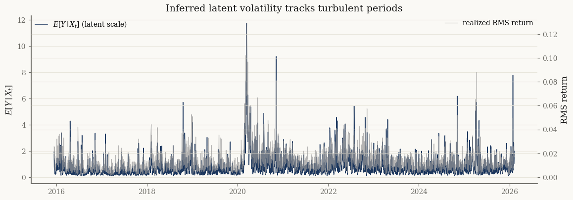
../../_images/6d241edf5ee8e878c4f4a4b89ed8f6392fe03dd0dd354a2c83eeea0e97eec0b8.png

corr(E[Y|X], realized RMS return) = 0.906

The strong correlation confirms the latent \(Y\) is doing exactly what it should: absorbing the time-varying volatility into the mixing variable.

Projecting to a portfolio#

Any linear combination of the assets is again a univariate member of the same family. project_portfolio returns that 1-D distribution in closed form — no re-fitting:

w = jnp.ones(len(basket)) / len(basket)         # equal weight
port = project_portfolio(model, w)
realized_port = R @ np.asarray(w)
print(f"portfolio mean  {float(port.mean()):.5f}  (empirical {realized_port.mean():.5f})")
print(f"portfolio std   {float(port.std()):.5f}  (empirical {realized_port.std():.5f})")
print(f"5% quantile     {float(port.ppf(jnp.array(0.05))):.5f}")

portfolio mean  0.00070  (empirical 0.00067)
portfolio std   0.01153  (empirical 0.01180)
5% quantile     -0.01750

Takeaways#

A full-\(\Sigma\) mixture fits real multivariate returns by EM; the log-likelihood ascent and fitted correlation are standard sanity checks.
\(\mathbb{E}[Y \mid X]\) recovered via joint.conditional_expectations is an interpretable latent volatility that tracks turbulent days.
project_portfolio(model, w) gives the portfolio return distribution in closed form for any weights.

Next: Factor mixtures for a Dow Jones 30 portfolio scales this to 30 assets with a low-rank factor covariance.

A multivariate stock basket

Contents