Normal variance-mean mixtures

The four named mixtures — VarianceGamma, NormalInverseGamma, NormalInverseGaussian, and GeneralizedHyperbolic — share one structure and one API. Each has a marginal layer (the distribution of \(X\), what you usually interact with) and a joint layer (the pair \((X, Y)\) with the latent subordinator, used by the EM E-step). This tutorial exercises both layers.

import jax
jax.config.update("jax_enable_x64", True)
import jax.numpy as jnp
import numpy as np

from normix import (
    VarianceGamma, NormalInverseGamma,
    NormalInverseGaussian, GeneralizedHyperbolic,
)
from normix.utils.plotting import set_theme

set_theme()
np.set_printoptions(precision=4, suppress=True)

A common constructor

All four marginals build from the location \(\mu\), the skewness vector \(\gamma\), a covariance \(\Sigma\), and the subordinator’s own parameters:

mu = jnp.array([0.0, 0.0])
gamma = jnp.array([0.3, -0.4])
Sigma = jnp.array([[1.0, 0.3], [0.3, 1.0]])

models = {
    "VarianceGamma": VarianceGamma.from_classical(
        mu=mu, gamma=gamma, sigma=Sigma, alpha=1.5, beta=1.5),
    "NormalInverseGamma": NormalInverseGamma.from_classical(
        mu=mu, gamma=gamma, sigma=Sigma, alpha=3.0, beta=2.0),
    "NormalInverseGaussian": NormalInverseGaussian.from_classical(
        mu=mu, gamma=gamma, sigma=Sigma, mu_ig=1.0, lam=1.5),
    "GeneralizedHyperbolic": GeneralizedHyperbolic.from_classical(
        mu=mu, gamma=gamma, sigma=Sigma, p=-0.5, a=1.0, b=1.0),
}
for name, m in models.items():
    print(f"{name:24s} mean={np.asarray(m.mean())}  d={m.d}")

VarianceGamma            mean=[ 0.3 -0.4]  d=2
NormalInverseGamma       mean=[ 0.3 -0.4]  d=2
NormalInverseGaussian    mean=[ 0.3 -0.4]  d=2
GeneralizedHyperbolic    mean=[ 0.3 -0.4]  d=2

Mean, covariance, and density

The marginal layer reports the moments of \(X\) (which fold in the variance-mean coupling through \(\gamma\)) and evaluates log_prob / pdf on single observations:

nig = models["NormalInverseGaussian"]
print("mean:\n", np.asarray(nig.mean()))
print("cov:\n", np.asarray(nig.cov()))
print("log_prob at origin:", float(nig.log_prob(jnp.zeros(2))))

mean:
 [ 0.3 -0.4]
cov:
 [[1.06   0.22  ]
 [0.22   1.1067]]
log_prob at origin: -1.382585051529043

Marginal vs joint layers

The .joint attribute exposes the \((X, Y)\) structure. The joint sampler returns both; the marginal sampler returns only \(X\) (the same draws, with \(Y\) dropped):

X, Y = nig.joint.rvs(20_000, seed=0)
print("X:", X.shape, " Y (subordinator):", Y.shape)
print("E[Y] =", float(Y.mean()))

sub = nig.joint.subordinator()       # the latent InverseGaussian
print("subordinator:", type(sub).__name__, " mean:", float(sub.mean()))

X: (20000, 2)  Y (subordinator): (20000,)
E[Y] = 1.0036306784108049
subordinator: InverseGaussian  mean: 1.0

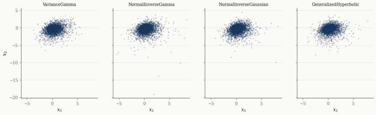
import matplotlib.pyplot as plt

fig, axes = plt.subplots(1, len(models), figsize=(14, 3.6), sharex=True, sharey=True)
for ax, (name, m) in zip(axes, models.items()):
    Xs = m.rvs(4000, seed=1)
    ax.scatter(np.asarray(Xs[:, 0]), np.asarray(Xs[:, 1]), s=3, alpha=0.2)
    ax.set_title(name, fontsize=9); ax.set_xlabel("$x_1$")
axes[0].set_ylabel("$x_2$")
plt.show()

The univariate face: CDF and quantiles

In one dimension the mixtures gain a scipy-style scalar API with cdf and ppf, useful for VaR-style tail calculations. Each marginal has a matching Univariate* class:

from normix import UnivariateNormalInverseGaussian

u = UnivariateNormalInverseGaussian.from_classical(
    mu=0.0, gamma=-0.5, sigma=1.0, mu_ig=1.0, lam=1.0)
print("mean / std :", float(u.mean()), float(u.std()))
print("5% quantile:", float(u.ppf(jnp.array(0.05))))
print("cdf(ppf):", float(u.cdf(u.ppf(jnp.array(0.05)))))

mean / std : -0.5 1.118033988749895
5% quantile: -2.4957660689683925
cdf(ppf): 0.05

Fitting by EM

fit runs the EM algorithm and returns an EMResult. Here we generate data from the NIG model and recover it:

X_train = nig.rvs(4000, seed=42)

init = NormalInverseGaussian.default_init(X_train)
result = init.fit(X_train, max_iter=100, tol=1e-3, verbose=0)

print("converged :", result.converged)
print("iterations:", result.n_iter)
print("elapsed   : %.2fs" % result.elapsed_time)
print("fitted γ  :", np.asarray(result.model.gamma))
print("true   γ  :", np.asarray(gamma))

converged : True
iterations: 57
elapsed   : 23.85s
fitted γ  : [ 0.3871 -0.3807]
true   γ  : [ 0.3 -0.4]

The returned EMResult.model is the fitted distribution; the EM machinery itself is covered in depth in the Batch EM in practice tutorial.

Takeaways

• The four marginals share from_classical(mu, gamma, sigma, <subordinator params>), mean/cov, pdf/log_prob, and rvs.

• .joint exposes the latent \((X, Y)\) pair and .joint.subordinator() the mixing distribution; joint.rvs returns both.

• Univariate* variants add cdf/ppf for \(d = 1\).

• fit performs EM and returns an EMResult whose .model is the fit.

Next: Factor mixtures for high dimensions scales these mixtures to high dimensions with a low-rank factor covariance.