InverseGaussian

The Inverse Gaussian (Wald) distribution on \((0, \infty)\) with mean \(\mu > 0\) and shape \(\lambda > 0\):

\[ f(x \mid \mu, \lambda) = \sqrt{\frac{\lambda}{2\pi}}\, x^{-3/2} \exp\!\left(-\frac{\lambda(x - \mu)^2}{2\mu^2 x}\right), \qquad x > 0. \]

It is exactly \(\mathrm{GIG}(p = -\tfrac12,\; a = \lambda/\mu^2,\; b = \lambda)\) and the subordinator behind the NormalInverseGaussian mixture — the workhorse heavy-tailed model for financial returns.

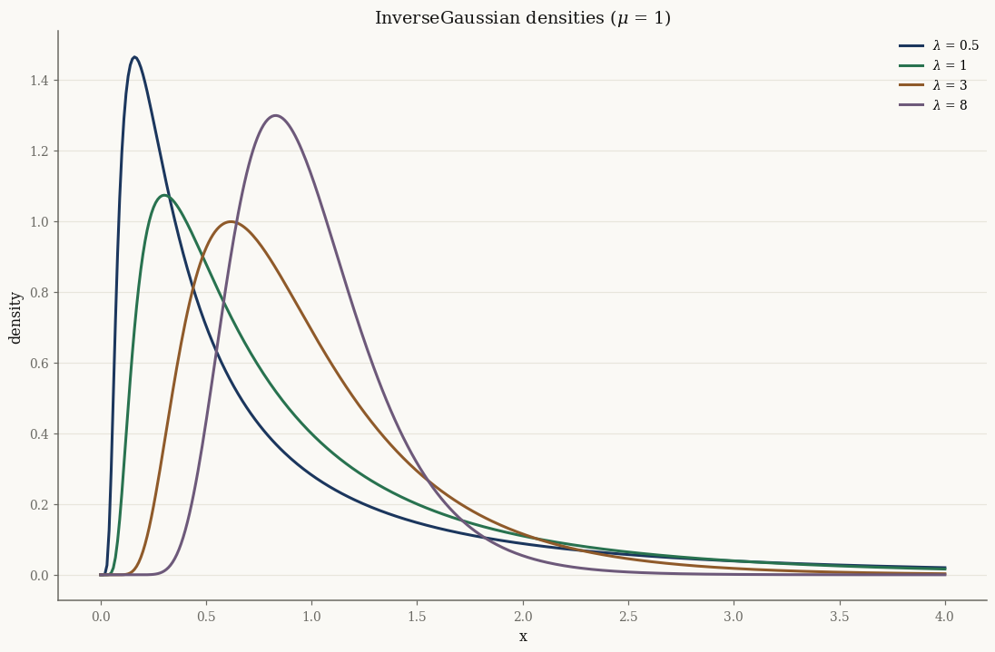
Density gallery

The shape \(\lambda\) controls concentration: as \(\lambda \to \infty\) the density concentrates around \(\mu\); small \(\lambda\) produces a heavy, right-skewed tail.

Show code cell source

Hide code cell source

import jax
jax.config.update("jax_enable_x64", True)
import jax.numpy as jnp
import numpy as np
import matplotlib.pyplot as plt

from normix import InverseGaussian
from normix.utils.plotting import set_theme

set_theme()
np.set_printoptions(precision=5, suppress=True)

x = jnp.linspace(1e-3, 4.0, 400)
fig, ax = plt.subplots()
for lam in [0.5, 1.0, 3.0, 8.0]:
    g = InverseGaussian(mu=jnp.array(1.0), lam=jnp.array(lam))
    ax.plot(np.asarray(x), np.asarray(jax.vmap(g.pdf)(x)), label=rf"$\lambda$ = {lam:g}")
ax.set_xlabel("x"); ax.set_ylabel("density")
ax.set_title(r"InverseGaussian densities ($\mu$ = 1)")
ax.legend()
plt.show()

Parametrizations

Stored attributes: mu, lam. Exponential family with sufficient statistic \(t(x) = [x,\; 1/x]\):

Parametrization	Value
Classical	mean \(\mu > 0\), shape \(\lambda > 0\)
Natural \(\theta\)	\([\,-\lambda/(2\mu^2),\; -\lambda/2\,]\)
Expectation \(\eta = \nabla\psi\)	\([\,\mu,\; 1/\mu + 1/\lambda\,] = (\mathbb{E}[X],\; \mathbb{E}[1/X])\)

The \(\eta \mapsto \theta\) inversion is closed-form: \(\mu = \eta_1\), \(\lambda = 1/(\eta_2 - 1/\eta_1)\).

Quick usage

ig = InverseGaussian(mu=jnp.array(1.0), lam=jnp.array(2.0))

print("mean/var/std:", float(ig.mean()), float(ig.var()), float(ig.std()))
print("cdf(1.0):    ", float(ig.cdf(jnp.array(1.0))))
print("5% quantile: ", float(ig.ppf(jnp.array(0.05))))

samples = ig.rvs(10_000, seed=0)           # Michael-Schucany-Haas sampler
fitted = InverseGaussian.fit_mle(samples)  # closed-form MLE
print("fit (mu,lam):", float(fitted.mu), float(fitted.lam))

mean/var/std: 1.0 0.5 0.7071067811865476
cdf(1.0):     0.6276978381552526
5% quantile:  0.28942800943818103
fit (mu,lam): 1.0052252606800098 2.0040649877504495

See also

• API: InverseGaussian

• Theory: The Generalized Inverse Gaussian Distribution — InverseGaussian as the \(p = -\tfrac12\) GIG

• Tutorial: Univariate positive distributions