MultivariateNormal

The Multivariate Normal on \(\mathbb{R}^d\) with mean \(\mu\) and covariance \(\Sigma\):

\[ f(x \mid \mu, \Sigma) = (2\pi)^{-d/2} |\Sigma|^{-1/2} \exp\!\left(-\tfrac12 (x - \mu)^\top \Sigma^{-1} (x - \mu)\right). \]

It is the Gaussian core of every mixture in this gallery: compounding it with a positive GIG subordinator (via \(X \mid Y \sim \mathcal{N}(\mu + \gamma Y,\; \Sigma Y)\)) produces the GeneralizedHyperbolic family. normix stores the lower Cholesky factor L_Sigma and routes all linear algebra through it — \(\Sigma^{-1}\) is never formed explicitly.

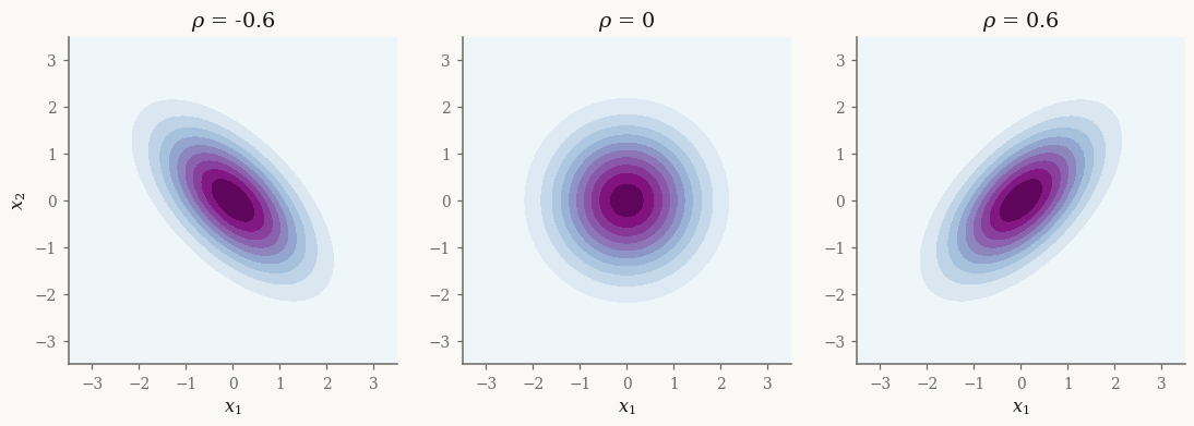
Density gallery

The correlation reshapes the elliptical contours; here are three \(2\times2\) covariances at \(\mu = 0\).

Show code cell source

Hide code cell source

import jax
jax.config.update("jax_enable_x64", True)
import jax.numpy as jnp
import numpy as np
import matplotlib.pyplot as plt

from normix import MultivariateNormal
from normix.utils.plotting import set_theme

set_theme()
np.set_printoptions(precision=5, suppress=True)

grid = jnp.linspace(-3.5, 3.5, 120)
GX, GY = jnp.meshgrid(grid, grid)
pts = jnp.stack([GX.ravel(), GY.ravel()], axis=1)

rhos = [-0.6, 0.0, 0.6]
fig, axes = plt.subplots(1, 3, figsize=(12, 4.0))
for ax, rho in zip(axes, rhos):
    Sigma = jnp.array([[1.0, rho], [rho, 1.0]])
    mvn = MultivariateNormal.from_classical(jnp.zeros(2), Sigma)
    Z = np.asarray(jax.vmap(mvn.pdf)(pts)).reshape(GX.shape)
    ax.contourf(np.asarray(GX), np.asarray(GY), Z, levels=10, cmap="BuPu")
    ax.set_title(rf"$\rho$ = {rho:g}")
    ax.set_aspect("equal"); ax.set_xlabel("$x_1$")
axes[0].set_ylabel("$x_2$")
plt.show()

Parametrizations

Stored attributes: mu \((d,)\) and L_Sigma \((d, d)\) (lower Cholesky of \(\Sigma\)). Exponential family with sufficient statistic \(t(x) = [x,\; \operatorname{vec}(xx^\top)]\):

Parametrization	Value
Classical	mean \(\mu \in \mathbb{R}^d\), covariance \(\Sigma \succ 0\)
Natural \(\theta\)	\([\,\Sigma^{-1}\mu,\; -\tfrac12\operatorname{vec}(\Sigma^{-1})\,]\)
Expectation \(\eta = \nabla\psi\)	\([\,\mu,\; \operatorname{vec}(\Sigma + \mu\mu^\top)\,] = (\mathbb{E}[X],\; \mathbb{E}[XX^\top])\)

Every conversion is analytical — no solver is invoked, and fit_mle is the closed-form sample mean and covariance.

Quick usage

mu = jnp.array([1.0, -0.5])
Sigma = jnp.array([[1.0, 0.4], [0.4, 2.0]])
mvn = MultivariateNormal.from_classical(mu, Sigma)

print("mean:\n", np.asarray(mvn.mean()))
print("cov:\n", np.asarray(mvn.cov()))
print("log_prob at mean:", float(mvn.log_prob(mu)))

samples = mvn.rvs(5_000, seed=0)           # (n, d)
fitted = MultivariateNormal.fit_mle(samples)
print("fitted mean:", np.asarray(fitted.mean()))

mean:
 [ 1.  -0.5]
cov:
 [[1.  0.4]
 [0.4 2. ]]
log_prob at mean: -2.1427598522197924
fitted mean: [ 0.97894 -0.51671]

See also

• API: MultivariateNormal

• Concepts: Exponential-family structure — the three parametrizations

• Tutorial: The multivariate normal