Divergences between models#

How far apart are two fitted distributions? normix provides two information divergences as first-class operations: the squared Hellinger distance \(H^2\) and the Kullback–Leibler divergence \(D_{\mathrm{KL}}\). Both have closed forms for exponential families in terms of the log-partition \(\psi\), so they are exact and differentiable — no Monte Carlo.

import jax
jax.config.update("jax_enable_x64", True)
import jax.numpy as jnp
import numpy as np

from normix import (
    Gamma, NormalInverseGaussian, GeneralizedHyperbolic,
    squared_hellinger, kl_divergence,
    squared_hellinger_from_psi, kl_divergence_from_psi,
)
from normix.utils.plotting import set_theme

set_theme()
np.set_printoptions(precision=5, suppress=True)

Hellinger and KL on distributions#

The convenience API takes two distributions of the same family:

p = Gamma(alpha=jnp.array(2.0), beta=jnp.array(1.5))
q = Gamma(alpha=jnp.array(2.5), beta=jnp.array(1.2))

print("H²(p, p) =", float(squared_hellinger(p, p)))   # identity → 0
print("H²(p, q) =", float(squared_hellinger(p, q)))
print("H²(q, p) =", float(squared_hellinger(q, p)))   # symmetric
print()
print("KL(p ‖ q) =", float(kl_divergence(p, q)))
print("KL(q ‖ p) =", float(kl_divergence(q, p)))       # asymmetric

H²(p, p) = 0.0
H²(p, q) = 0.057611811187182504
H²(q, p) = 0.057611811187182504

KL(p ‖ q) = 0.23114958120921036
KL(q ‖ p) = 0.24560834722128277

\(H^2\) is a bounded, symmetric distance in \([0, 1]\); KL is an asymmetric divergence in \([0, \infty)\). Hellinger is the better choice when you want a metric-like comparison between models.

The functional `*_from_psi` core#

The distribution-level functions are a thin layer over a functional core that works directly with the log-partition \(\psi\) and natural-parameter vectors. This is the layer the EM and optimization code calls internally:

squared_hellinger_from_psi(psi, theta_p, theta_q)
kl_divergence_from_psi(psi, grad_psi, theta_p, theta_q)

Feeding it a distribution’s own \(\psi\) reproduces the convenience result exactly:

psi = Gamma._log_partition_from_theta     # ψ(θ)
grad_psi = Gamma._grad_log_partition      # ∇ψ(θ) = η
theta_p, theta_q = p.natural_params(), q.natural_params()

print("H²  convenience :", float(squared_hellinger(p, q)))
print("H²  from_psi    :", float(squared_hellinger_from_psi(psi, theta_p, theta_q)))
print("KL  convenience :", float(kl_divergence(p, q)))
print("KL  from_psi    :", float(kl_divergence_from_psi(psi, grad_psi, theta_p, theta_q)))

H²  convenience : 0.057611811187182504
H²  from_psi    : 0.057611811187182504
KL  convenience : 0.23114958120921036
KL  from_psi    : 0.23114958120921036

Because the core takes a plain callable, you can differentiate through it — for example to take gradients of \(H^2\) with respect to natural parameters:

grad_H2 = jax.grad(lambda th: squared_hellinger_from_psi(psi, th, theta_q))(theta_p)
print("∂H²/∂θ_p =", np.asarray(grad_H2))

∂H²/∂θ_p = [-0.12021 -0.15706]

Hellinger as estimation error#

A natural use of \(H^2\) is to measure how far a fitted model is from the true one. As the sample size grows, the EM estimate converges and the Hellinger distance to the truth shrinks:

true = NormalInverseGaussian.from_classical(
    mu=jnp.array([0.0, 0.0]),
    gamma=jnp.array([0.4, -0.3]),
    sigma=jnp.array([[1.0, 0.3], [0.3, 1.0]]),
    mu_ig=1.0, lam=1.5)

ns = [250, 1000, 4000, 16000]
h2 = []
for n in ns:
    X = true.rvs(n, seed=0)
    fit = NormalInverseGaussian.default_init(X).fit(
        X, max_iter=120, tol=1e-4, e_step_backend="cpu").model
    h2.append(float(squared_hellinger(true, fit)))
    print(f"n = {n:6d}   H²(true, fit) = {h2[-1]:.5f}")

n =    250   H²(true, fit) = 0.02965
n =   1000   H²(true, fit) = 0.01043
n =   4000   H²(true, fit) = 0.00632
n =  16000   H²(true, fit) = 0.00355

import matplotlib.pyplot as plt

fig, ax = plt.subplots()
ax.loglog(ns, h2, "o-", label="$H^2(\\text{true}, \\hat{p}_n)$")
ax.loglog(ns, h2[0] * ns[0] / np.array(ns), "k--", lw=1, label="$\\propto 1/n$ reference")
ax.set_xlabel("sample size n"); ax.set_ylabel("squared Hellinger distance")
ax.set_title("Estimation error vs sample size")
ax.legend()
plt.show()

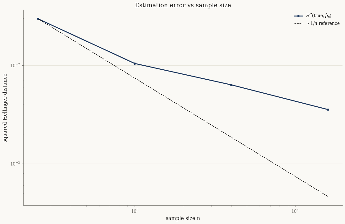
../../_images/14b30c85d0f23970e6420d262261c502cb091bf08728dee9a172b7ab1862aeb0.png

The fitted-model error tracks the \(1/n\) reference line — the expected parametric rate.

Note

For a mixture, squared_hellinger(p, q) returns the distance between the joint \((X, Y)\) distributions — which are exponential families with a closed-form \(\psi\) — not the marginal distance over \(X\) alone (the marginal is not an exponential family). The joint distance is an upper bound on the marginal one. Here true and fit are the same family with converging parameters, so both go to zero together; the trend is exactly what we want. But the gap matters when the latent parametrizations differ — see the next section.

Comparing across the GH family#

The Variance Gamma, Normal-Inverse Gamma, and Normal-Inverse Gaussian are all special cases of the Generalized Hyperbolic — they sit inside the GH family. normix makes that embedding explicit with to_generalized_hyperbolic, which re-expresses any of them in the GH parametrization (and hence the GH log-partition \(\psi\)):

data = true.rvs(4000, seed=0)
nig_fit = NormalInverseGaussian.default_init(data).fit(
    data, max_iter=120, tol=1e-4, e_step_backend="cpu").model
gh_fit = GeneralizedHyperbolic.default_init(data).fit(
    data, max_iter=120, tol=1e-4, e_step_backend="cpu").model

nig_as_gh = nig_fit.to_generalized_hyperbolic()   # NIG → GH, shared ψ
print("converted type:", type(nig_as_gh).__name__)

converted type: GeneralizedHyperbolic

Now both fits live in the same parametric family, so the closed-form divergence is defined. Since the NIG and GH fits to this data nearly coincide, the joint \((X, Y)\) Hellinger is small — and a Monte-Carlo estimate of the marginal Hellinger over \(X\) agrees, sitting just below it (the joint distance is always an upper bound on the marginal):

def marginal_h2_mc(p, q, n=200_000, seed=0):
    """Monte-Carlo squared Hellinger between the marginals of X."""
    Xp = p.rvs(n, seed=seed)
    log_ratio = jax.vmap(q.log_prob)(Xp) - jax.vmap(p.log_prob)(Xp)
    return float(1.0 - jnp.mean(jnp.exp(0.5 * log_ratio)))

print(f"joint    H²(nig→gh, gh) = {float(squared_hellinger(nig_as_gh, gh_fit)):.5f}")
print(f"marginal H²(nig,    gh) = {marginal_h2_mc(nig_fit, gh_fit):.5f}  (Monte Carlo)")

joint    H²(nig→gh, gh) = 0.00139
marginal H²(nig,    gh) = 0.00000  (Monte Carlo)

The lesson: the closed-form squared_hellinger is the right tool for comparing models of the same parametric form — an estimate vs its target, or two members embedded in the GH family via to_generalized_hyperbolic — where it is exact and cheap. Just remember it measures the joint \((X, Y)\) law: the bound is tight when the models nearly agree (as here) but can be loose when their latent subordinator parametrizations differ markedly. For ranking different families purely as fits to data — where only the marginal law of \(X\) matters — prefer out-of-sample log-likelihood (see A heavy-tailed index series) or the Monte-Carlo marginal Hellinger above.

Takeaways#

squared_hellinger(p, q) is a bounded symmetric distance; kl_divergence(p, q) is an asymmetric divergence — both closed-form for exponential families.
The *_from_psi functional core takes \(\psi\) and natural-parameter vectors, is differentiable, and underlies the convenience API.
For mixtures the convenience functions use the joint \((X, Y)\) law — an upper bound on the marginal distance. Use to_generalized_hyperbolic to place NIG/VG/NInvG in a shared family, and prefer out-of-sample log-likelihood (or a Monte-Carlo marginal Hellinger) when ranking different families on data.

Next: Goodness of fit turns to per-sample diagnostics — QQ plots, CDF overlays, and KS tests — on synthetic and real data.

Divergences between models

Contents