The Generalized Inverse Gaussian

The GIG distribution with parameters \((p, a, b)\) has density on \((0, \infty)\)

\[ f(x) = \frac{(a/b)^{p/2}}{2\,K_p(\sqrt{ab})}\, x^{p-1} \exp\!\Big(-\tfrac12\big(a x + b/x\big)\Big), \]

where \(K_p\) is the modified Bessel function of the second kind. Two features set it apart from the simpler positive distributions: its log-partition involves Bessel functions, and inverting expectation parameters back to natural parameters requires a multi-start Newton solver.

import jax
jax.config.update("jax_enable_x64", True)
import jax.numpy as jnp
import numpy as np

from normix import GIG, log_kv
from normix.utils.plotting import set_theme

set_theme()
np.set_printoptions(precision=5, suppress=True)

Construction, moments, density

gig = GIG(p=jnp.array(1.5), a=jnp.array(2.0), b=jnp.array(1.5))
print("mean =", float(gig.mean()), " var =", float(gig.var()), " std =", float(gig.std()))

q = jnp.array([0.1, 0.5, 0.9])
print("quantiles:", np.asarray(jax.vmap(gig.ppf)(q)))

mean = 2.0490381056766616  var = 1.674038105676659  std = 1.2938462449907482
quantiles: [0.72363 1.74949 3.7666 ]

import matplotlib.pyplot as plt

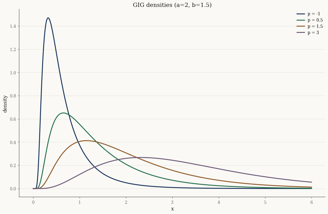
x = jnp.linspace(1e-3, 6.0, 400)
fig, ax = plt.subplots()
for p in [-1.0, 0.5, 1.5, 3.0]:
    g = GIG(p=jnp.array(p), a=jnp.array(2.0), b=jnp.array(1.5))
    ax.plot(np.asarray(x), np.asarray(jax.vmap(g.pdf)(x)), label=f"p = {p:g}")
ax.set_xlabel("x"); ax.set_ylabel("density")
ax.set_title("GIG densities (a=2, b=1.5)")
ax.legend()
plt.show()

A Bessel-valued log-partition

The normaliser is \(\psi(\theta) \propto \log K_p(\sqrt{ab})\), so the log-partition is evaluated through log_kv. Its gradient is the expectation parameter vector \(\eta = \mathbb{E}[t(X)] = (\mathbb{E}[\log X],\, \mathbb{E}[1/X],\, \mathbb{E}[X])\), which we can confirm by Monte Carlo:

eta = gig.expectation_params()
samples = gig.rvs(200_000, seed=0)
t = jax.vmap(GIG.sufficient_statistics)(samples)   # (log x, 1/x, x)
print("eta  (analytic) :", np.asarray(eta))
print("E[t(X)] (MC)    :", np.asarray(t.mean(axis=0)))

eta  (analytic) : [0.52583 0.73205 2.04904]
E[t(X)] (MC)    : [0.52941 0.73031 2.05684]

Because the gradient threads through log_kv, the derivative recurrences of the Bessel function (see Bessel functions and log_kv) are what make this exact and differentiable.

Inverting \(\eta \mapsto \theta\) with multi-start

Recovering natural parameters from moments is a strictly convex problem, but the Bessel terms make it stiff. from_expectation runs a Newton solver from several \(\eta\)-rescaled starting points and keeps the best. fit_mle chains moment-matching with this solve:

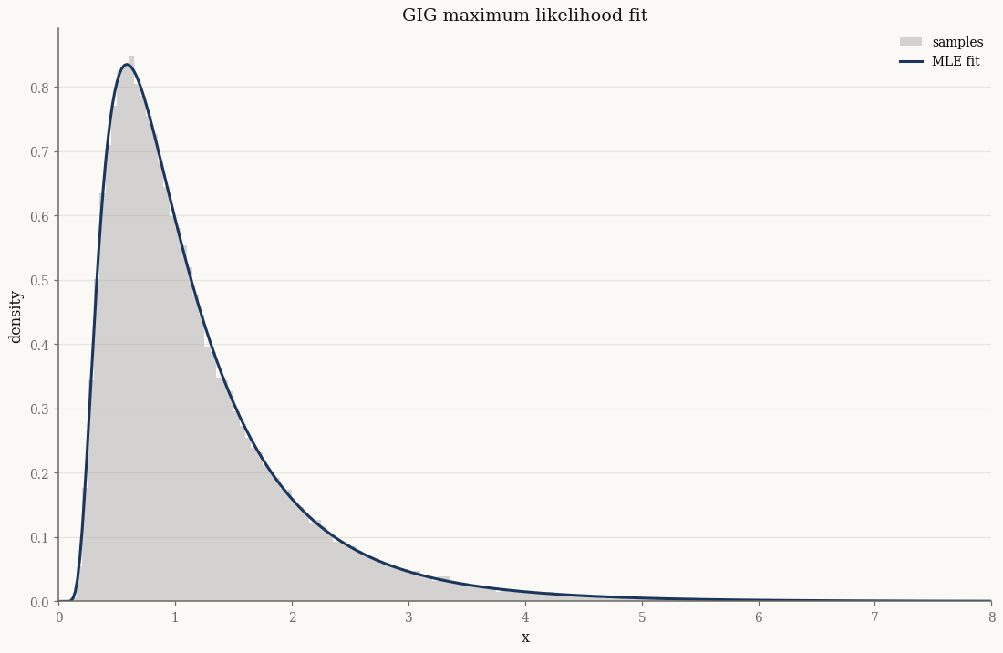
gig_true = GIG(p=jnp.array(-0.7), a=jnp.array(1.5), b=jnp.array(2.5))
X = gig_true.rvs(100_000, seed=1)

fitted = GIG.fit_mle(X)
print("true  (p, a, b):", float(gig_true.p), float(gig_true.a), float(gig_true.b))
print("MLE   (p, a, b):", float(fitted.p), float(fitted.a), float(fitted.b))

true  (p, a, b): -0.7 1.5 2.5
MLE   (p, a, b): -0.7731510073382721 1.4578868477899438 2.5712596518615825

fig, ax = plt.subplots()
ax.hist(np.asarray(X), bins=160, density=True, range=(0, 8),
        alpha=0.4, color="0.6", label="samples")
xg = jnp.linspace(1e-3, 8.0, 400)
ax.plot(np.asarray(xg), np.asarray(jax.vmap(fitted.pdf)(xg)), lw=2, label="MLE fit")
ax.set_xlim(0, 8); ax.set_xlabel("x"); ax.set_ylabel("density")
ax.set_title("GIG maximum likelihood fit")
ax.legend()
plt.show()

Two exact samplers

The GIG accepts a method for rvs. The Devroye ratio-of-uniforms sampler is the robust default; the PINV numerical inversion is competitive when drawing many samples from a fixed parameter set. Both reproduce the analytic moments:

print(f"{'method':>9s}  {'mean':>8s}  {'var':>8s}")
print(f"{'analytic':>9s}  {float(gig.mean()):8.4f}  {float(gig.var()):8.4f}")
for method in ["devroye", "pinv"]:
    s = gig.rvs(200_000, seed=2, method=method)
    print(f"{method:>9s}  {float(s.mean()):8.4f}  {float(s.var()):8.4f}")

   method      mean       var
 analytic    2.0490    1.6740
  devroye    2.0493    1.6778
     pinv    2.0508    1.6762

Takeaways

• The GIG log-partition is Bessel-valued, evaluated via log_kv; its gradient gives \(\eta = (\mathbb{E}[\log X], \mathbb{E}[1/X], \mathbb{E}[X])\).

• from_expectation uses an \(\eta\)-rescaled multi-start Newton solver to invert moments robustly; fit_mle wraps it.

• rvs offers "devroye" and "pinv" exact samplers.

Next: The multivariate normal moves to the multivariate Gaussian and its Cholesky parametrization.