The multivariate normal

The MultivariateNormal is the Gaussian core that every mixture in normix sits on top of. It is parametrized by a mean \(\mu\) and the lower Cholesky factor \(L_\Sigma\) of the covariance, \(\Sigma = L_\Sigma L_\Sigma^\top\). Storing the Cholesky factor (rather than \(\Sigma\) or \(\Sigma^{-1}\)) keeps every operation in terms of triangular solves — numerically stable and cheap.

import jax
jax.config.update("jax_enable_x64", True)
import jax.numpy as jnp
import numpy as np

from normix import MultivariateNormal
from normix.utils.plotting import set_theme

set_theme()
np.set_printoptions(precision=4, suppress=True)

Construction

You can build from classical \((\mu, \Sigma)\) or directly from the Cholesky factor. The two are equivalent:

mu = jnp.array([1.0, -0.5, 2.0])
Sigma = jnp.array([
    [1.0, 0.5, 0.2],
    [0.5, 2.0, 0.3],
    [0.2, 0.3, 1.5],
])

mvn = MultivariateNormal.from_classical(mu, Sigma)
mvn2 = MultivariateNormal(mu=mu, L_Sigma=jnp.linalg.cholesky(Sigma))

print("dimension d =", mvn.d)
print("Σ recovered:\n", np.asarray(mvn.cov()))
print("same model:", bool(jnp.allclose(mvn.L_Sigma, mvn2.L_Sigma)))

dimension d = 3
Σ recovered:
 [[1.  0.5 0.2]
 [0.5 2.  0.3]
 [0.2 0.3 1.5]]
same model: True

Log-density via triangular solves

log_prob evaluates the Gaussian log-density for a single observation by solving \(L_\Sigma z = (x - \mu)\) instead of inverting \(\Sigma\). We confirm it against the textbook formula:

x = jnp.array([0.3, 0.1, 1.7])
logp = mvn.log_prob(x)

d = mu.shape[0]
diff = x - mu
ref = -0.5 * (diff @ jnp.linalg.solve(Sigma, diff)
              + jnp.linalg.slogdet(Sigma)[1]
              + d * jnp.log(2 * jnp.pi))
print("log_prob      :", float(logp))
print("reference     :", float(ref))

log_prob      : -3.7459042876721753
reference     : -3.7459042876721753

Batch it with jax.vmap:

X = mvn.rvs(5, seed=0)
print("batched log_prob:", np.asarray(jax.vmap(mvn.log_prob)(X)))

batched log_prob: [-5.1962 -3.3081 -3.9871 -5.37   -6.4849]

Exponential-family round-trip

The Gaussian is an exponential family with closed-form natural and expectation parameters, so from_expectation is a direct conversion (no iterative solve):

theta = mvn.natural_params()
eta = mvn.expectation_params()
mvn_back = MultivariateNormal.from_expectation(eta)
print("μ recovered:", np.asarray(mvn_back.mean()))
print("Σ matches  :", bool(jnp.allclose(mvn_back.cov(), Sigma, atol=1e-8)))

μ recovered: [ 1.  -0.5  2. ]
Σ matches  : True

Sampling and maximum likelihood

rvs returns an (n, d) array; fit_mle recovers the empirical mean and covariance:

X = mvn.rvs(100_000, seed=3)
fitted = MultivariateNormal.fit_mle(X)
print("‖μ̂ − μ‖   =", float(jnp.linalg.norm(fitted.mean() - mu)))
print("‖Σ̂ − Σ‖_F =", float(jnp.linalg.norm(fitted.cov() - Sigma)))

‖μ̂ − μ‖   = 0.00564794607357663
‖Σ̂ − Σ‖_F = 0.011938651034048153

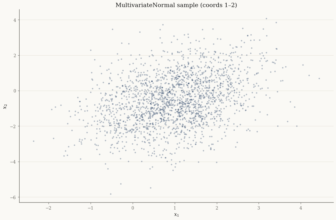
import matplotlib.pyplot as plt

fig, ax = plt.subplots()
ax.scatter(np.asarray(X[:2000, 0]), np.asarray(X[:2000, 1]), s=5, alpha=0.25)
ax.set_xlabel("$x_1$"); ax.set_ylabel("$x_2$")
ax.set_title("MultivariateNormal sample (coords 1–2)")
plt.show()

Takeaways

• MultivariateNormal stores \(\mu\) and the Cholesky factor L_Sigma; build it with from_classical(mu, sigma) or the constructor directly.

• log_prob uses triangular solves on \(L_\Sigma\) — stable and fast — and batches via jax.vmap.

• As an exponential family it has closed-form from_expectation, so fit_mle returns the empirical mean/covariance immediately.

Next: Normal variance-mean mixtures layers a positive subordinator on this Gaussian to build the full GH-family marginals.