A tour of the GH family

The Generalized Hyperbolic (GH) distribution and its relatives are all normal variance-mean mixtures: a Gaussian whose mean and covariance are scaled by a positive latent variable \(Y\),

\[ X \mid Y \sim \mathcal{N}(\mu + \gamma\, Y,\; \Sigma\, Y), \qquad Y \sim \text{subordinator}. \]

Different choices of the subordinator \(Y\) produce the whole family. This tutorial maps that hierarchy and shows how the pieces fit together.

import jax
jax.config.update("jax_enable_x64", True)
import jax.numpy as jnp
import numpy as np

from normix import (
    Gamma, InverseGamma, InverseGaussian, GIG,
    UnivariateVarianceGamma, UnivariateNormalInverseGamma,
    UnivariateNormalInverseGaussian, UnivariateGeneralizedHyperbolic,
)
from normix.utils.plotting import set_theme

set_theme()
np.set_printoptions(precision=5, suppress=True)

The mixing mechanism

Sampling is hierarchical: draw \(Y\), then draw \(X\) given \(Y\). We can reproduce a marginal sample by hand and check it matches the built-in sampler. The joint rvs returns both \(X\) and the latent \(Y\):

gh = UnivariateGeneralizedHyperbolic.from_classical(
    mu=0.0, gamma=0.4, sigma=1.0, p=-0.5, a=1.0, b=1.0)

X, Y = gh.joint.rvs(50_000, seed=0)
print("X shape:", X.shape, " Y shape:", Y.shape)
print("E[Y] =", float(Y.mean()), "  Var[Y] =", float(Y.var()))
print("skew(X) =", float(((X - X.mean())**3).mean() / X.std()**3))

X shape: (50000, 1)  Y shape: (50000,)
E[Y] = 1.0080074760677304   Var[Y] = 1.0118961918124396
skew(X) = 1.137510856845186

The positive skew of \(X\) comes entirely from \(\gamma\): the variance-mean coupling tilts the Gaussian by an amount proportional to \(Y\).

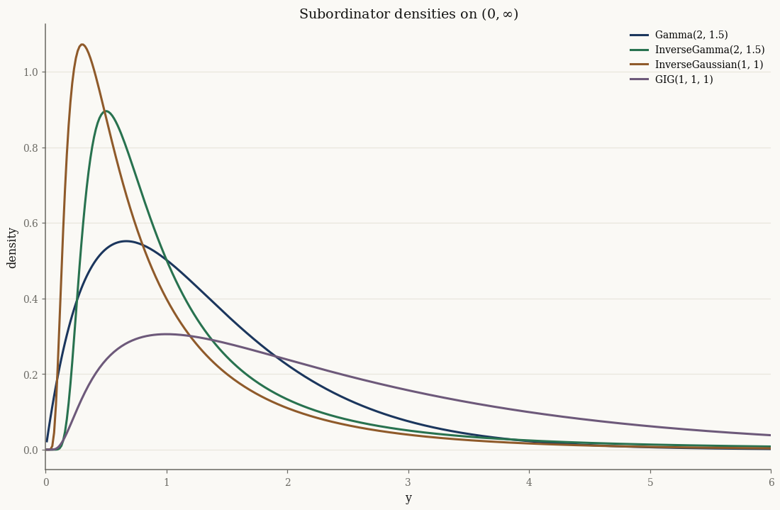
Four subordinators

The subordinator is itself an exponential family. The four building blocks are Gamma, InverseGamma, InverseGaussian, and the GIG (Generalized Inverse Gaussian) that nests them all:

subs = {
    "Gamma(2, 1.5)": Gamma(alpha=jnp.array(2.0), beta=jnp.array(1.5)),
    "InverseGamma(2, 1.5)": InverseGamma(alpha=jnp.array(2.0), beta=jnp.array(1.5)),
    "InverseGaussian(1, 1)": InverseGaussian(mu=jnp.array(1.0), lam=jnp.array(1.0)),
    "GIG(1, 1, 1)": GIG(p=jnp.array(1.0), a=jnp.array(1.0), b=jnp.array(1.0)),
}

import matplotlib.pyplot as plt
y = jnp.linspace(0.01, 6.0, 400)
fig, ax = plt.subplots()
for name, s in subs.items():
    ax.plot(np.asarray(y), np.asarray(jax.vmap(s.pdf)(y)), label=name)
ax.set_xlabel("y"); ax.set_ylabel("density"); ax.set_xlim(0, 6)
ax.set_title("Subordinator densities on $(0, \\infty)$")
ax.legend()
plt.show()

The GIG nests the others

The GIG distribution with parameters \((p, a, b)\) has density on \((0,\infty)\) proportional to \(y^{p-1}\exp\!\big(-\tfrac12(a y + b/y)\big)\). Its degenerate limits recover the simpler subordinators exactly:

Limit	Recovers
\(b \to 0,\ p > 0\)	\(\mathrm{Gamma}(p,\, a/2)\)
\(a \to 0,\ p < 0\)	\(\mathrm{InverseGamma}(-p,\, b/2)\)
\(p = -\tfrac12\)	\(\mathrm{InverseGaussian}\)

x = jnp.linspace(0.05, 6.0, 300)

def max_logp_gap(d1, d2):
    return float(jnp.max(jnp.abs(jax.vmap(d1.log_prob)(x) - jax.vmap(d2.log_prob)(x))))

# b -> 0, p > 0  =>  Gamma(p, a/2)
gap_gamma = max_logp_gap(
    GIG(p=jnp.array(2.0), a=jnp.array(3.0), b=jnp.array(1e-8)),
    Gamma(alpha=jnp.array(2.0), beta=jnp.array(1.5)))

# a -> 0, p < 0  =>  InverseGamma(-p, b/2)
gap_invgamma = max_logp_gap(
    GIG(p=jnp.array(-2.0), a=jnp.array(1e-8), b=jnp.array(3.0)),
    InverseGamma(alpha=jnp.array(2.0), beta=jnp.array(1.5)))

# p = -1/2  =>  InverseGaussian(mu, lam) with a = lam/mu^2, b = lam
mu_, lam_ = 1.5, 2.0
gap_invgauss = max_logp_gap(
    GIG(p=jnp.array(-0.5), a=jnp.array(lam_ / mu_**2), b=jnp.array(lam_)),
    InverseGaussian(mu=jnp.array(mu_), lam=jnp.array(lam_)))

print(f"GIG -> Gamma       max|Δ log p| = {gap_gamma:.2e}")
print(f"GIG -> InverseGamma max|Δ log p| = {gap_invgamma:.2e}")
print(f"GIG -> InvGaussian  max|Δ log p| = {gap_invgauss:.2e}")

GIG -> Gamma       max|Δ log p| = 9.25e-08
GIG -> InverseGamma max|Δ log p| = 2.25e-08
GIG -> InvGaussian  max|Δ log p| = 4.44e-15

The four marginal mixtures

Choosing each subordinator for the mixing variable yields a named marginal distribution:

Subordinator	Marginal	normix class
Gamma	Variance Gamma	VarianceGamma
Inverse Gamma	Normal-Inverse Gamma	NormalInverseGamma
Inverse Gaussian	Normal-Inverse Gaussian	NormalInverseGaussian
GIG	Generalized Hyperbolic	GeneralizedHyperbolic

We compare them in 1-D against a standard normal, all centred and scaled to unit variance, to expose the differences in the tails:

marginals = {
    "VarianceGamma": UnivariateVarianceGamma.from_classical(
        mu=0.0, gamma=0.0, sigma=1.0, alpha=1.2, beta=1.2),
    "NormalInverseGamma": UnivariateNormalInverseGamma.from_classical(
        mu=0.0, gamma=0.0, sigma=1.0, alpha=3.0, beta=2.0),
    "NormalInverseGaussian": UnivariateNormalInverseGaussian.from_classical(
        mu=0.0, gamma=0.0, sigma=1.0, mu_ig=1.0, lam=1.0),
    "GeneralizedHyperbolic": UnivariateGeneralizedHyperbolic.from_classical(
        mu=0.0, gamma=0.0, sigma=1.0, p=-0.5, a=1.0, b=1.0),
}
for name, m in marginals.items():
    print(f"{name:24s}  mean={float(m.mean()):+.3f}  std={float(m.std()):.3f}")

VarianceGamma             mean=+0.000  std=1.000
NormalInverseGamma        mean=+0.000  std=1.000
NormalInverseGaussian     mean=+0.000  std=1.000
GeneralizedHyperbolic     mean=+0.000  std=1.000

from jax.scipy.stats import norm

xs = jnp.linspace(-6, 6, 600)
fig, axes = plt.subplots(1, 2, figsize=(12, 4.6))
for name, m in marginals.items():
    pdf = np.asarray(jax.vmap(m.pdf)(xs))
    axes[0].plot(np.asarray(xs), pdf, label=name)
    axes[1].plot(np.asarray(xs), np.log(pdf + 1e-300), label=name)
for ax in axes:
    ax.plot(np.asarray(xs), np.asarray(norm.pdf(xs)) if ax is axes[0]
            else np.asarray(norm.logpdf(xs)),
            "k--", lw=1.2, label="Normal(0, 1)")
    ax.set_xlabel("x")
axes[0].set_ylabel("density"); axes[0].set_title("Densities")
axes[1].set_ylabel("log density"); axes[1].set_title("Log densities (tail view)")
axes[1].set_ylim(-18, 0)
axes[0].legend(fontsize=8)
plt.show()

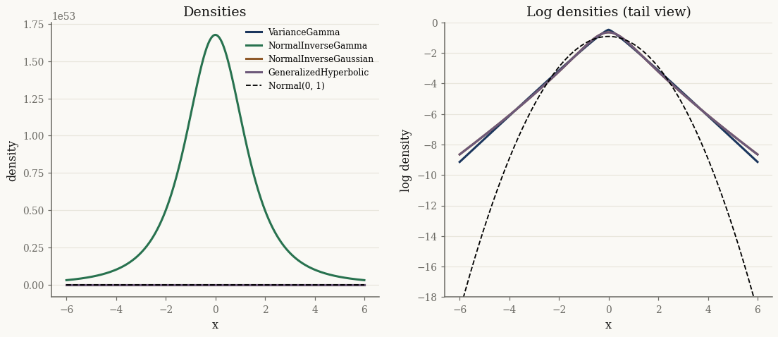
The log-density panel makes the point: every GH-family marginal has heavier tails than the Gaussian. Mixing over a positive \(Y\) is exactly what produces the excess kurtosis seen in financial returns and other heavy-tailed data.

Takeaways

• The GH family is the set of normal variance-mean mixtures \(X \mid Y \sim \mathcal{N}(\mu + \gamma Y, \Sigma Y)\).

• The subordinator \(Y\) selects the member: Gamma → VG, Inverse Gamma → NInvG, Inverse Gaussian → NIG, GIG → GH.

• The GIG nests Gamma, InverseGamma, and InverseGaussian as limits, so GH nests all the others.

• Asymmetry comes from \(\gamma\); heavy tails come from the mixing.

Next: Bessel functions and log_kv digs into the Bessel function log_kv that makes the GH densities computable, and Random sampling covers drawing samples from every distribution.