Batch EM in practice#

Fitting a normal variance-mean mixture is a missing-data problem: the subordinator \(Y\) is latent. The EM algorithm alternates

E-step — given the current model, compute the conditional expectations \(\mathbb{E}[t(Y) \mid X]\) of the sufficient statistics, and
M-step — set the new expectation parameters \(\eta\) to those conditional means and convert \(\eta \mapsto \theta\) via from_expectation.

BatchEMFitter runs this loop over the full dataset each iteration. This tutorial covers its diagnostics, regularizations, and backend options.

import jax
jax.config.update("jax_enable_x64", True)
import jax.numpy as jnp
import numpy as np

from normix import NormalInverseGaussian
from normix.fitting.em import BatchEMFitter
from normix.utils.plotting import set_theme

set_theme()
np.set_printoptions(precision=4, suppress=True)

Data and a fitter#

We simulate from a known 3-D NIG model and fit it back. BatchEMFitter.fit returns an EMResult:

true = NormalInverseGaussian.from_classical(
    mu=jnp.array([0.0, 0.0, 0.0]),
    gamma=jnp.array([0.4, -0.3, 0.1]),
    sigma=jnp.array([[1.0, 0.3, 0.1], [0.3, 1.0, 0.2], [0.1, 0.2, 1.0]]),
    mu_ig=1.0, lam=1.5)
X = true.rvs(5000, seed=0)

init = NormalInverseGaussian.default_init(X)
fitter = BatchEMFitter(
    max_iter=150, tol=1e-4, verbose=1,
    e_step_backend="cpu", m_step_backend="cpu", m_step_method="newton")
result = fitter.fit(init, X)

print("converged :", result.converged)
print("iterations:", result.n_iter)
print("elapsed   : %.2fs" % result.elapsed_time)

============================================================
  EM Fitting: NormalInverseGaussian
============================================================
  Algorithm    : EM
  Loop         : Python loop
  E-step       : cpu
  M-step       : cpu / newton
  Regularize   : none
  Tolerance    : 1.0e-04
  Max iters    : 150
  Converged after 56 iterations (16.44s), final LL=-4.129249
converged : True
iterations: 56
elapsed   : 16.44s

The EMResult is a frozen record:

print("fields:", [f for f in result.__dataclass_fields__])
print("fitted γ:", np.asarray(result.model.gamma))
print("true   γ:", np.asarray(true.gamma))

fields: ['model', 'log_likelihoods', 'param_changes', 'n_iter', 'converged', 'elapsed_time']
fitted γ: [ 0.4167 -0.339   0.082 ]
true   γ: [ 0.4 -0.3  0.1]

Convergence diagnostics#

With verbose >= 1 the result carries the per-iteration log-likelihood history and the maximum relative parameter change. Both should improve monotonically and flatten at convergence:

import matplotlib.pyplot as plt

ll = np.asarray(result.log_likelihoods)
pc = np.asarray(result.param_changes)

fig, (a0, a1) = plt.subplots(1, 2, figsize=(12, 4.4))
a0.plot(np.arange(1, len(ll) + 1), ll)
a0.set_xlabel("iteration"); a0.set_ylabel("mean log-likelihood")
a0.set_title("Log-likelihood ascent")
a1.semilogy(np.arange(1, len(pc) + 1), pc)
a1.axhline(fitter.tol, color="0.5", ls="--", lw=1, label="tol")
a1.set_xlabel("iteration"); a1.set_ylabel("max relative param change")
a1.set_title("Parameter change"); a1.legend()
plt.show()

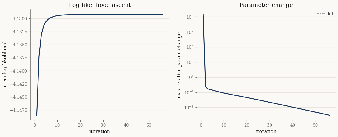
../../_images/c35c7b42438177d2f0f10f95843b9e55327f57e4ed81eddd02a40ad0cbf79468.png

EM never decreases the likelihood — a useful invariant when debugging a fit.

Regularizations#

Mixtures are only identified up to a scale split between \(\Sigma\) and the subordinator. BatchEMFitter accepts a regularization to pin that gauge:

Value	Constraint
`'none'`	unconstrained
`'det_sigma_one'`	\(\lvert\Sigma\rvert = 1\)
`'det_sigma_x'`	\(\lvert\Sigma\rvert = \lvert\Sigma_0\rvert\) (initial value)
`'a_eq_b'`	GIG subordinator with \(a = b\)

With det_sigma_one the fitted scale matrix has unit determinant (check model.sigma(), the scale \(\Sigma\), not the marginal covariance):

fitter_reg = BatchEMFitter(
    max_iter=150, tol=1e-4, regularization="det_sigma_one",
    e_step_backend="cpu", m_step_backend="cpu")
res_reg = fitter_reg.fit(init, X)
print("det Σ (regularized):", float(jnp.linalg.det(res_reg.model.sigma())))
print("log|Σ|             :", float(res_reg.model.log_det_sigma()))

det Σ (regularized): 1.0000000000000004
log|Σ|             : 3.41740524767431e-16

CPU and JAX backends#

The E-step is dominated by Bessel evaluations and the M-step by the \(\eta \mapsto \theta\) solve. Each can run on a JAX or a CPU/scipy backend independently:

e_step_backend="cpu" routes Bessel through scipy.special.kve — a large speedup for the GIG/NIG E-step on CPU.
m_step_backend="cpu" uses the numpy/scipy Newton solver for the subordinator update; m_step_method selects "newton", "lbfgs", or "bfgs".

Backends change how the arithmetic runs, not the answer:

res_jax = BatchEMFitter(
    max_iter=150, tol=1e-4,
    e_step_backend="jax", m_step_backend="cpu").fit(init, X)

mll_cpu = float(result.model.marginal_log_likelihood(X))
mll_jax = float(res_jax.model.marginal_log_likelihood(X))
print(f"mean log-lik  (cpu E-step): {mll_cpu:.6f}")
print(f"mean log-lik  (jax E-step): {mll_jax:.6f}")

mean log-lik  (cpu E-step): -4.129249
mean log-lik  (jax E-step): -4.129249

The convenience wrapper#

model.fit(X, ...) is a thin wrapper that builds a BatchEMFitter with the same keywords and calls fitter.fit(self, X) — convenient for one-off fits. Reach for BatchEMFitter directly when you need an eta_update rule (see Incremental (mini-batch) EM) or want to reuse a configured fitter.

result2 = init.fit(X, max_iter=150, tol=1e-4, e_step_backend="cpu")
print("same fit:", bool(jnp.allclose(result2.model.gamma, result.model.gamma, atol=1e-4)))

same fit: True

Takeaways#

EM alternates an E-step (conditional moments \(\mathbb{E}[t(Y) \mid X]\)) with an M-step (from_expectation); BatchEMFitter.fit returns an EMResult.
verbose >= 1 records the log-likelihood and parameter-change histories for diagnostics; the likelihood ascends monotonically.
regularization fixes the scale gauge; e_step_backend / m_step_backend / m_step_method tune performance without changing the optimum.

Next: Incremental (mini-batch) EM replaces the full-data sweep with mini-batches and stochastic \(\eta\)-update rules.

Batch EM in practice

Contents