The exponential family#

Every distribution in normix is an exponential family. A density in this class can be written

\[ p(x \mid \theta) = h(x)\, \exp\!\big(\langle \theta,\, t(x)\rangle - \psi(\theta)\big), \]

with three ingredients:

the log base measure \(\log h(x)\),
the sufficient statistics \(t(x)\),
the log-partition function \(\psi(\theta)\) (the normaliser).

This single structure gives us three interchangeable parametrizations and a uniform recipe for moments, maximum likelihood, and the EM algorithm. This tutorial walks through that structure on the simplest member of the family — the Gamma distribution.

import jax
jax.config.update("jax_enable_x64", True)
import jax.numpy as jnp
import numpy as np

from normix import Gamma
from normix.utils.plotting import set_theme

set_theme()
np.set_printoptions(precision=5, suppress=True)

A distribution as a pytree#

A normix distribution is an immutable equinox.Module. We build a Gamma from its classical shape/rate parameters \((\alpha, \beta)\):

dist = Gamma(alpha=jnp.array(2.0), beta=jnp.array(1.0))
dist.mean(), dist.var(), dist.std()

(Array(2., dtype=float64),
 Array(2., dtype=float64),
 Array(1.41421, dtype=float64))

The log-density acts on a single observation; batch it with jax.vmap:

x = jnp.linspace(0.1, 8.0, 200)
log_p = jax.vmap(dist.log_prob)(x)
pdf = jax.vmap(dist.pdf)(x)
float(jnp.max(jnp.abs(jnp.exp(log_p) - pdf)))  # pdf == exp(log_prob)

0.0

Three parametrizations#

The classical parameters map to natural parameters \(\theta\) and to expectation parameters \(\eta = \nabla\psi(\theta) = \mathbb{E}[t(X)]\). normix exposes all three and converts between them losslessly:

theta = dist.natural_params()        # natural θ
eta = dist.expectation_params()      # expectation η = ∇ψ(θ) = E[t(X)]
print("theta =", np.asarray(theta))
print("eta   =", np.asarray(eta))

theta = [ 1. -1.]
eta   = [0.42278 2.     ]

# Round-trip: classical → θ → classical and classical → η → classical
d_from_theta = Gamma.from_natural(theta)
d_from_eta = Gamma.from_expectation(eta)
print("from_natural:    ", float(d_from_theta.alpha), float(d_from_theta.beta))
print("from_expectation:", float(d_from_eta.alpha), float(d_from_eta.beta))

from_natural:     2.0 1.0
from_expectation: 2.0000000000000036 1.0000000000000018

from_expectation is the workhorse of the M-step: it inverts \(\eta \mapsto \theta\) by solving a strictly convex problem, so any valid moment vector \(\eta\) produces a well-defined distribution.

\(\eta\) really is \(\mathbb{E}[t(X)]\)#

The expectation parameters are not an abstraction — they are the mean of the sufficient statistics. We can check this by Monte Carlo:

samples = dist.rvs(200_000, seed=0)
t = jax.vmap(Gamma.sufficient_statistics)(samples)   # t(x) = [log x, x] for Gamma
print("E[t(X)] empirical:", np.asarray(t.mean(axis=0)))
print("eta (analytic)   :", np.asarray(eta))

E[t(X)] empirical: [0.42388 2.00414]
eta (analytic)   : [0.42278 2.     ]

Fisher information is the curvature of \(\psi\)#

The Hessian \(\nabla^2\psi(\theta)\) is the Fisher information, and it equals the covariance of the sufficient statistics. normix computes it analytically:

I = dist.fisher_information()
print("I(theta) = Hessian of psi:\n", np.asarray(I))
print("\nCov[t(X)] empirical:\n", np.cov(np.asarray(t), rowvar=False))

I(theta) = Hessian of psi:
 [[0.64493 1.     ]
 [1.      2.     ]]

Cov[t(X)] empirical:
 [[0.64901 1.00491]
 [1.00491 2.01102]]

JAX and CPU backends#

Moments derived from \(\psi\) come in two interchangeable backends: a JIT-able JAX path (the default) and a numpy/scipy CPU path used inside the EM hot loop. They agree to numerical precision:

eta_jax = dist.expectation_params(backend="jax")
eta_cpu = dist.expectation_params(backend="cpu")
float(jnp.max(jnp.abs(eta_jax - jnp.asarray(eta_cpu))))

0.0

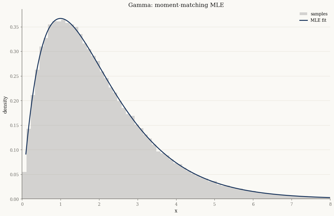
Maximum likelihood is one line#

Because the MLE of an exponential family matches moments (\(\hat\eta = \frac{1}{n}\sum_i t(x_i)\), then \(\hat\theta\) via from_expectation), fitting is a single call:

fitted = Gamma.fit_mle(samples)
print("true  (alpha, beta):", float(dist.alpha), float(dist.beta))
print("MLE   (alpha, beta):", float(fitted.alpha), float(fitted.beta))

true  (alpha, beta): 2.0 1.0
MLE   (alpha, beta): 1.9933564529024204 0.9946213764711547

import matplotlib.pyplot as plt

fig, ax = plt.subplots()
ax.hist(np.asarray(samples), bins=120, density=True, alpha=0.4,
        label="samples", color="0.6")
ax.plot(np.asarray(x), np.asarray(jax.vmap(fitted.pdf)(x)), label="MLE fit")
ax.set_xlim(0, 8)
ax.set_xlabel("x")
ax.set_ylabel("density")
ax.set_title("Gamma: moment-matching MLE")
ax.legend()
plt.show()

../../_images/791e899b21e4dd8100aa59ae5399ce4f458de0b24ce2aed905c2a49e5b87007a.png

Takeaways#

A normix distribution is defined by \(\big(\log h,\, t,\, \psi\big)\) and stored as an immutable pytree.
Three parametrizations — classical, natural \(\theta\), expectation \(\eta\) — convert via natural_params, expectation_params, from_natural, from_expectation.
\(\eta = \nabla\psi(\theta) = \mathbb{E}[t(X)]\) and \(\nabla^2\psi(\theta) = \operatorname{Cov}[t(X)]\) is the Fisher information.
Every moment and the MLE follow from \(\psi\), with matching JAX and CPU backends.

Next: A tour of the GH family shows how all the richer distributions are built on top of this base by mixing a normal over a positive subordinator.

The exponential family

Contents