InverseGamma

The Inverse Gamma distribution on \((0, \infty)\) with shape \(\alpha > 0\) and rate \(\beta > 0\):

\[ f(x \mid \alpha, \beta) = \frac{\beta^\alpha}{\Gamma(\alpha)}\, x^{-\alpha-1} e^{-\beta/x}, \qquad x > 0. \]

If \(X \sim \mathrm{Gamma}(\alpha, \beta)\) then \(1/X \sim \mathrm{InvGamma}(\alpha, \beta)\). It is the \(a \to 0\) limit of the GIG and the subordinator behind the NormalInverseGamma mixture. The right tail is polynomial, so the mean exists only for \(\alpha > 1\) and the variance only for \(\alpha > 2\).

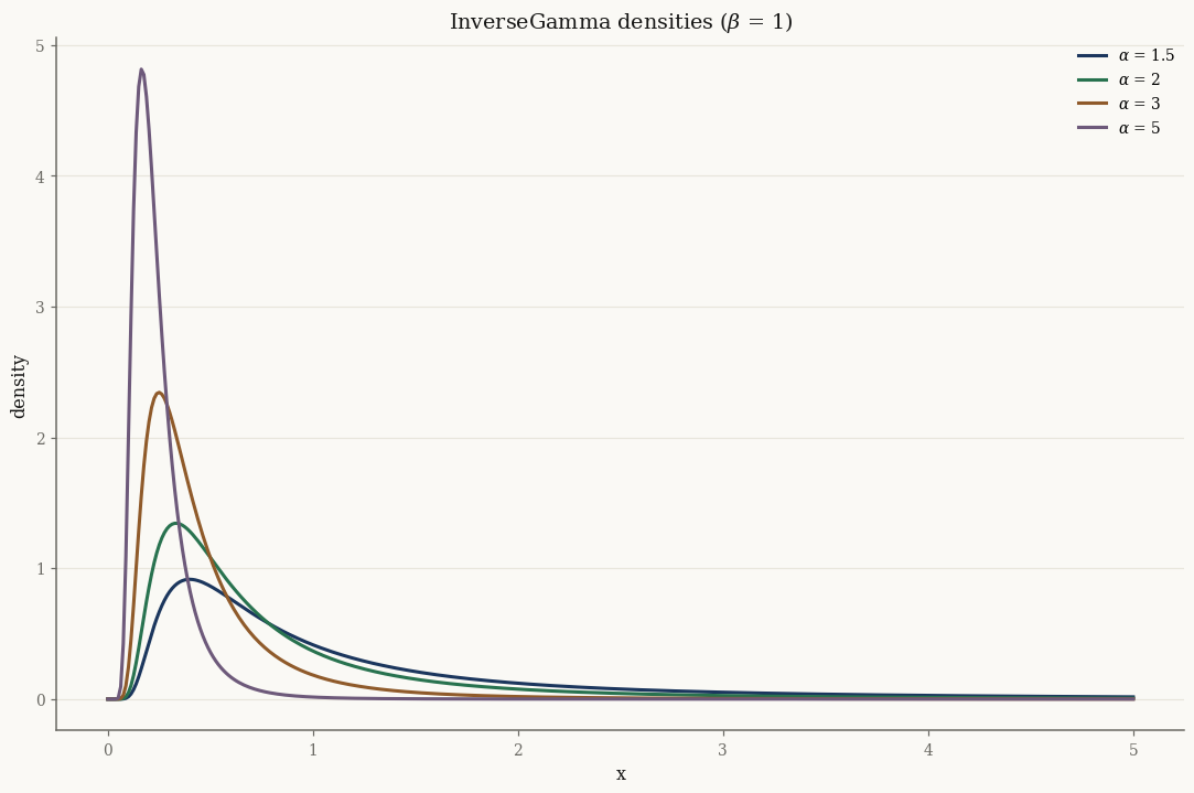
Density gallery

Smaller \(\alpha\) makes the right tail heavier; the mode sits at \(\beta/(\alpha+1)\), well below the mean.

Show code cell source

Hide code cell source

import jax
jax.config.update("jax_enable_x64", True)
import jax.numpy as jnp
import numpy as np
import matplotlib.pyplot as plt

from normix import InverseGamma
from normix.utils.plotting import set_theme

set_theme()
np.set_printoptions(precision=5, suppress=True)

x = jnp.linspace(1e-3, 5.0, 400)
fig, ax = plt.subplots()
for alpha in [1.5, 2.0, 3.0, 5.0]:
    g = InverseGamma(alpha=jnp.array(alpha), beta=jnp.array(1.0))
    ax.plot(np.asarray(x), np.asarray(jax.vmap(g.pdf)(x)), label=rf"$\alpha$ = {alpha:g}")
ax.set_xlabel("x"); ax.set_ylabel("density")
ax.set_title(r"InverseGamma densities ($\beta$ = 1)")
ax.legend()
plt.show()

Parametrizations

Stored attributes: alpha, beta. Exponential family with sufficient statistic \(t(x) = [-1/x,\; \log x]\):

Parametrization	Value
Classical	shape \(\alpha > 0\), rate \(\beta > 0\)
Natural \(\theta\)	\([\,\beta,\; -(\alpha + 1)\,]\)
Expectation \(\eta = \nabla\psi\)	\([\,-\alpha/\beta,\; \log\beta - \psi(\alpha)\,] = (\mathbb{E}[-1/X],\; \mathbb{E}[\log X])\)

where \(\psi\) is the digamma function.

Quick usage

ig = InverseGamma(alpha=jnp.array(3.0), beta=jnp.array(2.0))

print("mean/var/std:", float(ig.mean()), float(ig.var()), float(ig.std()))
print("cdf(1.0):    ", float(ig.cdf(jnp.array(1.0))))
print("95% quantile:", float(ig.ppf(jnp.array(0.95))))

samples = ig.rvs(10_000, seed=0)
fitted = InverseGamma.fit_mle(samples)     # moment-matching MLE
print("fit (a,b):   ", float(fitted.alpha), float(fitted.beta))

mean/var/std: 1.0 1.0 1.0
cdf(1.0):     0.6766764161830632
95% quantile: 2.4459103821334023
fit (a,b):    3.0051761339255814 2.0008877634257516

See also

• API: InverseGamma

• Theory: The Generalized Inverse Gaussian Distribution — InverseGamma as a limit of the GIG family

• Tutorial: Univariate positive distributions