Your first model, step by step

The Quickstart showed the whole loop at once. Here we slow down and walk through each stage — constructing a distribution, sampling from it, fitting one back, and checking the result — so the pieces and their shapes are clear.

import jax
jax.config.update("jax_enable_x64", True)
import jax.numpy as jnp
import numpy as np

from normix import NormalInverseGaussian
from normix.utils.plotting import set_theme

set_theme()
np.set_printoptions(precision=4, suppress=True)

1. Build a distribution from parameters

We start with a known 2-D Normal-Inverse Gaussian so we have a ground truth to recover. It is specified by a location \(\mu\), a skewness vector \(\gamma\), a covariance \(\Sigma\), and the subordinator parameters \((\mu_{IG}, \lambda)\):

truth = NormalInverseGaussian.from_classical(
    mu=jnp.array([0.0, 0.0]),
    gamma=jnp.array([0.6, -0.4]),       # asymmetry
    sigma=jnp.array([[1.0, 0.5], [0.5, 1.5]]),
    mu_ig=1.0, lam=1.2)

print("mean:", np.asarray(truth.mean()))
print("cov:\n", np.asarray(truth.cov()))

mean: [ 0.6 -0.4]
cov:
 [[1.3    0.3   ]
 [0.3    1.6333]]

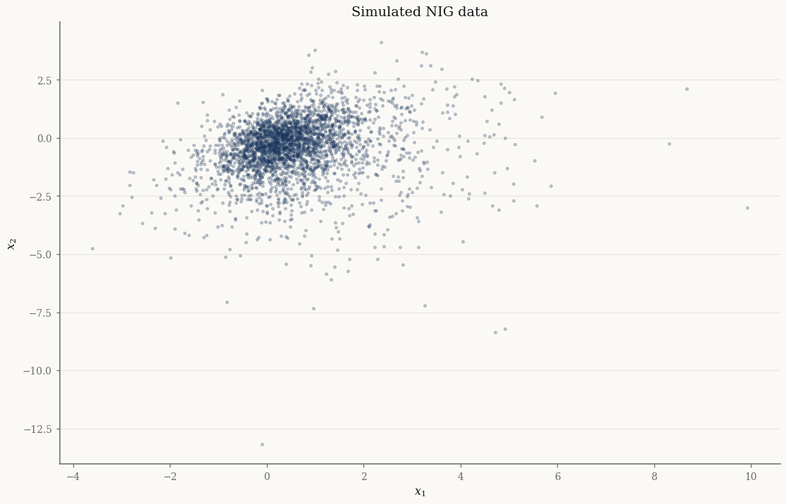
2. Sample some data

rvs(n, seed) returns an (n, d) array. This stands in for whatever data you would fit in practice:

X = truth.rvs(3000, seed=0)
print("data shape:", X.shape)

data shape: (3000, 2)

import matplotlib.pyplot as plt

fig, ax = plt.subplots()
ax.scatter(np.asarray(X[:, 0]), np.asarray(X[:, 1]), s=6, alpha=0.25)
ax.set_xlabel("$x_1$"); ax.set_ylabel("$x_2$")
ax.set_title("Simulated NIG data")
plt.show()

3. Initialize and fit

default_init builds a starting model from the data’s moments — you never have to guess initial parameters. fit then runs EM and returns an EMResult:

init = NormalInverseGaussian.default_init(X)
result = init.fit(X, max_iter=150, tol=1e-4, verbose=1, e_step_backend="cpu")
fitted = result.model

print(f"converged: {result.converged} in {result.n_iter} iterations")
print("fitted gamma:", np.asarray(fitted.gamma), " (true [0.6, -0.4])")

============================================================
  EM Fitting: NormalInverseGaussian
============================================================
  Algorithm    : EM
  Loop         : Python loop
  E-step       : cpu
  M-step       : cpu / newton
  Regularize   : none
  Tolerance    : 1.0e-04
  Max iters    : 150
  Converged after 70 iterations (18.36s), final LL=-2.947356
converged: True in 70 iterations
fitted gamma: [ 0.5437 -0.4973]  (true [0.6, -0.4])

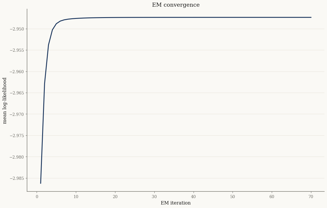
4. Check the fit

A good fit recovers the parameters and assigns high likelihood. We compare the fitted mean/covariance to the truth and look at the log-likelihood ascent:

print(f"‖mean − true‖  = {float(jnp.linalg.norm(fitted.mean() - truth.mean())):.4f}")
print(f"‖cov − true‖_F = {float(jnp.linalg.norm(fitted.cov() - truth.cov())):.4f}")

fig, ax = plt.subplots()
ax.plot(np.arange(1, len(result.log_likelihoods) + 1), np.asarray(result.log_likelihoods))
ax.set_xlabel("EM iteration"); ax.set_ylabel("mean log-likelihood")
ax.set_title("EM convergence")
plt.show()

‖mean − true‖  = 0.0340
‖cov − true‖_F = 0.1038

5. Use the model

The fitted object is a full distribution. Evaluate densities, draw samples, or compute moments — all the same methods the true model has:

x0 = jnp.array([0.5, -0.5])
print("log density at x0:", float(fitted.log_prob(x0)))
print("new samples:", fitted.rvs(3, seed=99).shape)

log density at x0: -1.7235205345490745
new samples: (3, 2)

Recap

1. Construct with from_classical (or load real data and skip to step 3).

2. Sample with rvs(n, seed).

3. Initialize with default_init(X) and fit with fit(X, ...).

4. Inspect EMResult — model, converged, n_iter, log_likelihoods.

5. Use the fitted model’s log_prob, mean, cov, rvs, ….

From here, the Distributions guide helps you pick a family, and the Batch EM in practice tutorial goes deeper on the fitting machinery.