VarianceGamma

The Variance Gamma distribution is the normal variance-mean mixture

\[ X \mid Y \sim \mathcal{N}(\mu + \gamma Y,\; \Sigma Y), \qquad Y \sim \mathrm{Gamma}(\alpha, \beta), \]

with a Gamma subordinator — equivalently the GIG limit \(p = \alpha,\; a = 2\beta,\; b \to 0\). It has lighter tails than the other mixtures and no continuous component at the origin, making it a natural first choice for mildly heavy-tailed, possibly skewed data.

Density gallery

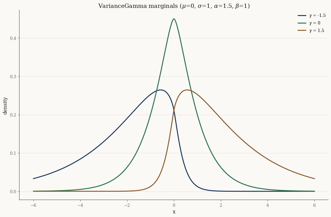
The skewness vector \(\gamma\) tilts the density; at \(\gamma = 0\) it is symmetric about \(\mu\). Below is the one-dimensional marginal.

Show code cell source

Hide code cell source

import jax
jax.config.update("jax_enable_x64", True)
import jax.numpy as jnp
import numpy as np
import matplotlib.pyplot as plt

from normix import VarianceGamma, UnivariateVarianceGamma
from normix.utils.plotting import set_theme

set_theme()
np.set_printoptions(precision=5, suppress=True)

x = jnp.linspace(-6.0, 6.0, 400)
fig, ax = plt.subplots()
for g in [-1.5, 0.0, 1.5]:
    vg = UnivariateVarianceGamma.from_classical(
        mu=0.0, gamma=g, sigma=1.0, alpha=1.5, beta=1.0)
    ax.plot(np.asarray(x), np.asarray(jax.vmap(vg.pdf)(x)), label=rf"$\gamma$ = {g:g}")
ax.set_xlabel("x"); ax.set_ylabel("density")
ax.set_title(r"VarianceGamma marginals ($\mu$=0, $\sigma$=1, $\alpha$=1.5, $\beta$=1)")
ax.legend()
plt.show()

Parametrizations

Built from the shared location/shape block and the Gamma subordinator:

Symbol	Attribute	Meaning
\(\mu\)	mu	location \((d,)\)
\(\gamma\)	gamma	skewness \((d,)\)
\(\Sigma = L_\Sigma L_\Sigma^\top\)	L_Sigma	dispersion Cholesky \((d, d)\)
\(\alpha\)	alpha	Gamma shape
\(\beta\)	beta	Gamma rate

The marginal \(f(x)\) is not itself an exponential family, but the joint \((X, Y)\) is — its natural parametrization \(\theta\) and the EM machinery are derived in The Generalized Hyperbolic Distribution.

Quick usage

Raw \((\gamma, \Sigma, \beta)\) are identified only up to the scale gauge \(Y \mapsto cY\) (see EM Algorithm for Generalized Hyperbolic Distributions); compare the invariants \(\mu\), \(\gamma E[Y]\), and \(E[Y]\,\Sigma\) instead.

mu = jnp.array([0.0, 0.0])
gamma = jnp.array([0.3, -0.4])
Sigma = jnp.array([[1.0, 0.3], [0.3, 1.0]])

vg = VarianceGamma.from_classical(mu=mu, gamma=gamma, sigma=Sigma, alpha=1.5, beta=1.5)
print("mean:", np.asarray(vg.mean()))
print("cov:\n", np.asarray(vg.cov()))

X = vg.rvs(2_000, seed=0)                  # (n, d); vg.joint.rvs gives (X, Y)
result = VarianceGamma.default_init(X).fit(X, max_iter=50, tol=1e-3)
fit = result.model
ey = float(fit.joint.subordinator().mean())
print("converged:", bool(result.converged), "n_iter:", int(result.n_iter))
print("mu:", np.asarray(fit.mu))
print("gamma * E[Y]:", np.asarray(fit.gamma) * ey)   # true [0.3, -0.4] (E[Y]=1)
print("E[Y] * Sigma:\n", ey * np.asarray(fit.sigma()))
print("mean:", np.asarray(fit.mean()))
print("cov:\n", np.asarray(fit.cov()))

mean: [ 0.3 -0.4]
cov:
 [[1.06    0.22   ]
 [0.22    1.10667]]
converged: True n_iter: 16
mu: [-0.00496  0.03692]
gamma * E[Y]: [ 0.29762 -0.41079]
E[Y] * Sigma:
 [[0.924   0.25254]
 [0.25254 0.96342]]
mean: [ 0.29267 -0.37387]
cov:
 [[0.98506 0.16826]
 [0.16826 1.07974]]

The \(d = 1\) sibling UnivariateVarianceGamma adds a scipy-style cdf / ppf; the high-dimensional FactorVarianceGamma swaps \(\Sigma\) for a factor model.

See also

• API: VarianceGamma

• Theory: The Generalized Hyperbolic Distribution

• Tutorial: Normal variance-mean mixtures