Two coordinates can have the same marginal distributions and quite different joint extremes. Density geometry compares their contours; this note constructs a joint law and asks which dependence summaries exist. The context is SCoFT v4 §§6.1–6.7, pp. 108–119 Taleb, 2025. The calculations below are derived here; the semicircle limit is a separately cited theorem.
We use dimension , location vector , positive definite scatter matrix , and Student degrees of freedom . Scatter specifies shape and scale; it is a covariance matrix only when we explicitly say so. Here is the identity matrix; all densities use Lebesgue measure. Symbols follow the shared notation.
A shared random scale¶
An elliptical law has characteristic function
for , where is a scalar function for which this is a characteristic function. The definition can allow positive semidefinite and singular laws; our density calculations use positive definite . It does not require moments or independence of coordinates.
Let , let be independent of , and choose . The normal variance-mixture construction extends to
Conditioning on proves ellipticality. It also proves when . For a deterministic matrix and vector , substitution of in the characteristic function gives location and scatter for . This proves closure under linear maps, including singular images. It does not assert that every stable vector is elliptical.
For example, let equal or with equal probabilities, . Covariance remains , whereas the density at is multiplied, relative to , by
Strict convexity of proves the inequality. This finite mixture has finite exponential moments in every direction: its MGF is an average of two Gaussian MGFs. Increased central density and kurtosis do not imply an asymptotic power tail.
The normalized Student law¶
Take a precision with gamma shape and rate both . Conditioning on gives the normal density with covariance . Writing , integration over gives
The gamma integral proves both the constant and normalization, since the integrated conditional densities each have mass one. Every nonzero linear projection is a univariate Student with the same , location , and scale . This follows directly from being normal, independent of the same .
The univariate moment gate therefore applies to each coordinate: a mean exists for , and finite covariance requires . Gamma integration gives
For , a finite sample scatter matrix can still be calculated; it does not estimate a finite population covariance matrix under this model.
Diagonal scatter does not give independence¶
Set , , and . The two marginal Student laws share their random precision. Bayes’ rule gives
Mixing the conditional normal for thus gives a Student law with degrees of freedom and scale . This scale varies with on sets of positive probability, which proves dependence for every finite . For the Pearson correlation is nevertheless zero. For , zero off-diagonal scatter is not a zero Pearson correlation: that population coefficient is undefined.
There is also a direct joint-tail test without moment assumptions. For , put , with the standard normal survival. Conditional independence gives
The variance is positive because is strictly increasing and the mixing law is nondegenerate. Independent Student coordinates have zero excess instead. These bounded indicator probabilities exist even for Cauchy marginals. They do not by themselves specify an asymptotic tail-dependence coefficient.
Mutual information without second moments¶
For a bivariate density with marginals , mutual information is
It is KL divergence from the joint law to the product of its marginals. The KL inequality gives nonnegativity and equality exactly at independence. No variance appears in the definition, but integrability must still be checked.
We derive the Student value. Write and let denote the digamma function, distinct from the shared canon’s log-partition symbol. In whitened polar coordinates, satisfies
Indeed the radial density is proportional to ; the displayed substitution gives the beta density. Differentiating its normalizing integral in the second parameter gives . The differentiation is justified on compact subsets of positive parameters by integrable endpoint powers times . The beta integral is the cited input (DLMF 5.12.1). Substitution into the normalized log density now proves
All these logarithmic expectations are finite for . Thus subtracting entropies is legitimate even when no second moment exists. For unit diagonal scatter and off-diagonal entry , ,
The determinant gives the first term; the earlier dependence proof gives strict positivity of the second. Independent rescaling of either coordinate cancels from the entropy difference. At , and , so nats. The Gaussian analogue has only . A single observed sample correlation near zero cannot establish independence in either model.
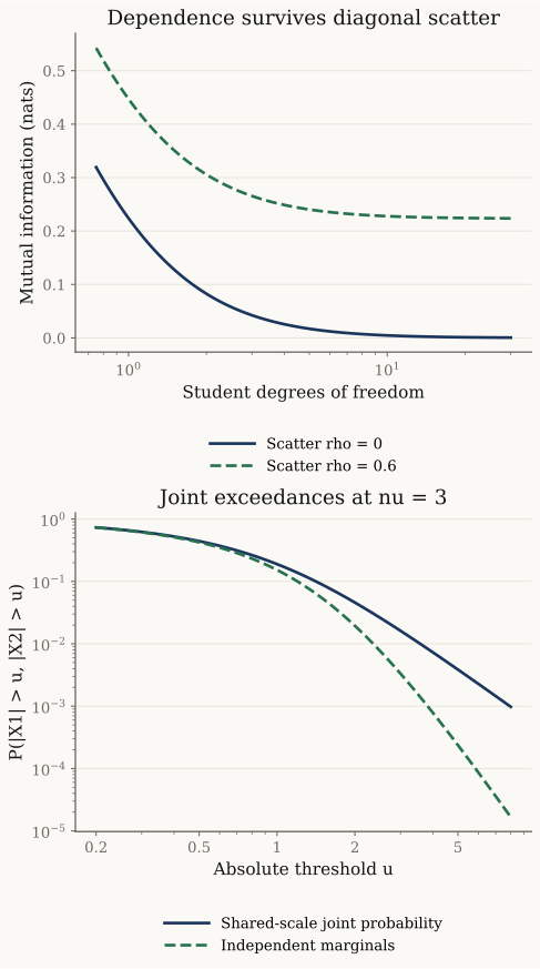
Population calculations, with no fitted data. The upper panel evaluates the entropy formula at and 0.6. The lower panel integrates over gamma precision at and ; the shared scale increases joint absolute exceedances above the independent-marginal probability. All displayed quantities are dimensionless; mutual information uses natural logarithms.
A bounded statistic need not have a population target¶
For two nonzero finite data vectors , the uncentered cosine is . Cauchy–Schwarz proves . Pearson’s sample correlation applies this formula to and and requires both vectors to be nonconstant. The two statistics are different. A constant column makes the centered coefficient undefined, rather than zero.
Hold observations fixed and replace the last pair by , where and . For the uncentered cosine the leading numerator is , and the norm product is . For the centered statistic, write . Here is the last coordinate unit vector and is the all-ones vector. The leading vectors are and with . Both coefficients therefore tend to as . This is a deterministic contamination limit at fixed sample size, not an iid sampling theorem.
Our repeated Student samples below compare and with scatter parameter . Only the latter has population Pearson correlation 0.6. Sampling quantiles quantify this finite experiment; they are neither confidence intervals nor a universal convergence rate.
What the matrix ensemble must specify¶
Let be the upper-left block of one infinite real symmetric matrix, with independent identically distributed entries on and above the diagonal, mean zero and variance one, mirrored below it. The semicircle theorem says that the empirical eigenvalue measure of converges weakly almost surely to density on . This is a cited result, not proved here: Tao, 254A Notes 4, Theorem 1 and §1 truncation reduction. Finite variance suffices for this empirical-measure limit; an infinite fourth moment does not automatically invalidate it. Convergence of the largest eigenvalue is a different question.
Two finite identities explain the sensitivity to a large entry. For any real symmetric matrix with eigenvalues ,
Orthogonal diagonalization proves the first identity, and proves the second. A single large entry therefore forces a large spectral radius. Neither identity proves a limiting heavy-tail spectral law. Nor does a Wigner theorem apply directly to a sample covariance matrix , with a centered data matrix; that matrix is positive semidefinite and has a different construction.
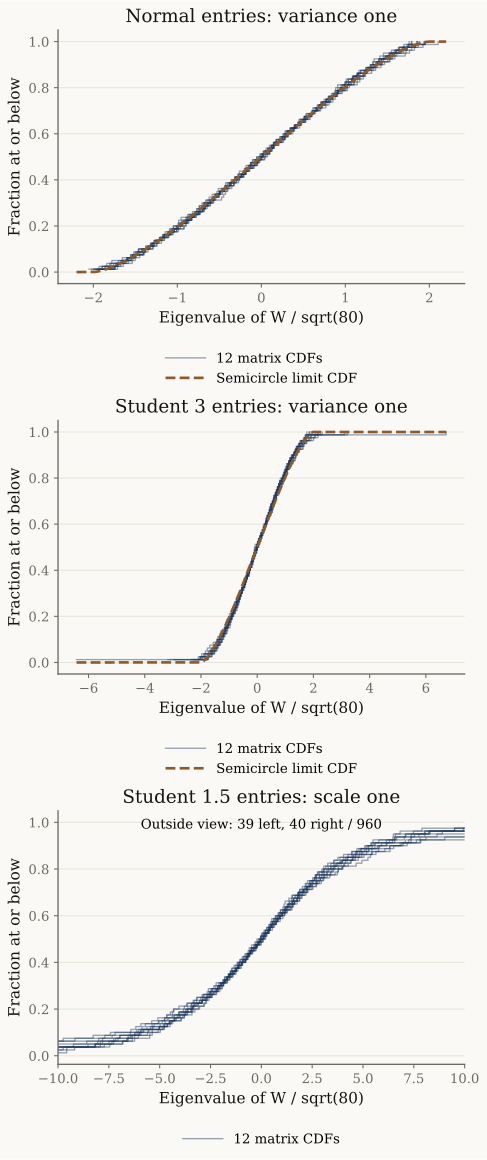
Twelve independent symmetric matrices per law, all divided by . Each thin curve is a matrix’s empirical CDF, computed from all 80 eigenvalues. The Student-1.5 viewport is ; 39 eigenvalues lie below it and 40 above it, out of 960 across all twelve matrices. The CDFs keep those values in their ranks and denominators. The normal and Student-3 entries have variance one; Student 1.5 has unit Student scale and infinite variance. The common divisor in the last panel is a finite comparison convention, not a proposed limit scaling. The dashed semicircle CDF appears only in the two finite-variance panels.
Regression with a stated population target¶
Consider and an independent error with and . Define the response ; the letter remains reserved for mixing variance. Independence gives
For iid pairs, the strong law applied to proves that sample correlation squared converges almost surely to this value. The product is integrable by Cauchy–Schwarz. In a fitted simple ordinary least-squares regression with an intercept and nonconstant columns, write for centered sums. The normal equations give and fitted centered response . Its sum of squares is , so fitted . This proves the connection to the population target. For the expectation statement, extend by zero on samples with a constant column. The strong law makes both denominators positive eventually almost surely; this bounded extension therefore satisfies by bounded convergence. The coefficient on a degenerate sample itself remains undefined. The convergence argument supplies no error or universal upward-bias claim.
Use sample_correlation.
from xmath.incerto.multivariate import sample_correlation

print(f"Constant centered column: {sample_correlation([1, 1, 1], [1, 2, 3]):.4g}")
print(f"Zero uncentered column: {sample_correlation([0, 0, 0], [1, 2, 3], centered=False):.4g}")
print(f"Nondegenerate columns: {sample_correlation([1, 2, 3], [2, 4, 6]):.4g}")
Output
Constant centered column: nan
Zero uncentered column: nan
Nondegenerate columns: 1
For Student error with scale and , . At , , the target is . The fourth error moment is infinite, so the ordinary variance-based CLT for empirical second moments cannot be used; the strong-law argument still works. When , this population Pearson target is undefined. Letting a finite-variance family’s decrease to two sends its target to zero, but does not define a correlation at the boundary.
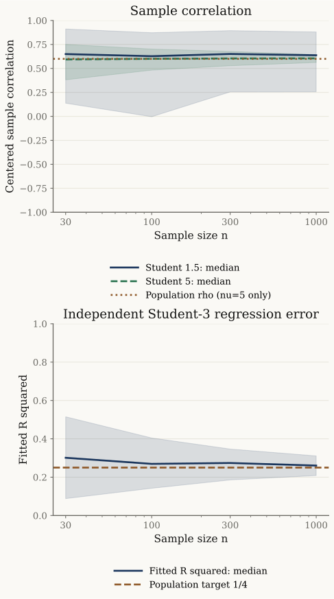
PCG64 seed 20261018, 400 replications at each size 30, 100, 300, 1000. Upper panel: bivariate Students with common scale and scatter parameter 0.6; the dotted population line applies only to . Lower panel: response , independent normal , and unit-scale Student-3 error; the population target is . Bands describe sampling variation, not Monte Carlo confidence intervals. No draw is clipped or removed.
Reproduce and read further¶
Use bivariate_student, sample_correlation, student_mutual_information.
import numpy as np
from xmath.incerto.multivariate import (
    bivariate_student, sample_correlation, student_mutual_information,
)

rng = np.random.default_rng(20261020)
for nu in (1.5, 5):
    sample = bivariate_student(rng, nu, rho=0, size=2000)
    print(f"nu={nu:.4g}, sample r: {sample_correlation(*sample.T):.3f}")
    print(f"Population information: {student_mutual_information(nu):.4g}")
Output
nu=1.5, sample r: -0.098
Population information: 0.1281
nu=5, sample r: -0.036
Population information: 0.01713
Diagonal scatter gives zero population correlation only for here; at that population coefficient is undefined.
Figure regeneration: uv run python demos/incerto/multivariate_tails.py. It prints the
finite-model calculations, quadrature errors and sampling quantiles, and
creates these three figures plus the linked geometry and regime figures.
The API reference lists the tested helper module.
The chapter 6 guide maps all sections and appendix A;
moment estimation explains why existence,
estimator variance and convergence rate must be considered separately.
SCoFT v4 Taleb, 2025, §§6.1–6.3, pp. 108–114, motivates the mixture and independence questions; §6.4, pp. 114–115, motivates mutual information; §6.5, pp. 115–116, spectra; §6.6, pp. 116–117, sample correlation; and §6.7, pp. 117–119, regression. These are context locators. The source’s historical regressions and general portfolio prescriptions are not evidence for the models proved here.
- Taleb, N. N. (2025). Statistical Consequences of Fat Tails (3rd ed.). https://arxiv.org/abs/2001.10488v4