A finite sample produces a finite empirical moment in exact arithmetic. It does not establish that the corresponding population moment exists. Even when that moment exists, the estimator can have infinite variance or be dominated by events that most samples miss. We separate these questions using an exact Pareto model and a finite Gaussian mixture.
The sample notation follows the shared canon. For iid and order , write
These are raw moments. For a signed variable, replace by ; a signed odd moment requires separate integrability conditions.
The estimator needs a higher moment¶
For Pareto with ,
Assume . Then the sample moment is unbiased for every , but it has finite variance only if . In that regime,
We prove both assertions. Linearity gives the expectation whenever is finite. For , independence makes the cross-covariances zero. For , nonnegativity gives , whose expectation is infinite. Since the estimator has finite mean, its variance is infinite too. Equality at is excluded by the logarithmic divergence of the Pareto moment integral.
For example, gives , but has infinite variance at every finite . At , , , and the estimator variance is . A simulated finite standard error in the first model cannot certify the population variance of the estimator.
Consistency does not require estimator variance¶
We prove convergence in probability when , without a finite th moment. Set and . For fixed , Chebyshev’s inequality gives convergence of the average of to its expectation, because these variables are bounded and iid. The omitted nonnegative part has expected average as . Markov’s inequality controls that average uniformly in . For any error tolerance, first choose to make this expectation small, then to control the bounded average. The triangle inequality proves in probability. This argument supplies no uniform rate over all integrable laws.
When , the stronger almost-sure divergence follows from the nonnegative infinite-mean theorem, applied to . That linked note proves the result by truncation. Finite observed values and floating-point overflow are separate matters; neither determines which population regime applies.
A square root changes the moment question¶
Let . If , then
The identity is immediate from the definition. Cauchy–Schwarz gives the inequality and integrability of ; hence its variance is finite. Thus infinite variance of the empirical second moment does not imply infinite variance of the empirical root mean square. For the sample standard deviation , the identity gives the same finite-second-moment conclusion for . A fixed correction for does not change this conclusion.
The square root can introduce downward bias through concavity. The sample raw moment remains unbiased. Bias, estimator variance, and the frequency of an underestimate are different properties.
A comparison under an exact Gaussian model¶
Here we know the center is zero and assume iid , with . Compare the root mean square with the Gaussian-calibrated mean absolute deviation . Both target under these assumptions. We can compute their mean squared errors without simulation.
The normal absolute-moment integrals give and . For , changing variables from a normal density gives a gamma shape , scale 2 for each square. Independence and the gamma convolution identity give shape , scale 2 for . Integrating against that density yields
The last identity uses . The corresponding MSE for , divided by , is . These are exact finite- risks under squared-error loss, including ’s bias. The demo prints them for .
This comparison does not carry over unchanged to the rare-state mixture: , so the same now targets , whereas the population standard deviation is . Jensen’s inequality makes these unequal for nonconstant with finite mean. Changing the model can change both the sampling error and the target of a calibrated statistic.
Finite moments that most samples miss¶
Use the two-state variance mixture with , , and , with independent standard-normal . Draw the pairs independently. The population second moment is 1 and fourth moment is 77.25, so
The probability that no wide component is selected is . Conditional on that event, all observations are independent and the empirical second moment has expectation 0.5. At , this event has probability about 0.605. Rare samples compensate in the unconditional mean; the raw second moment estimator is still unbiased.
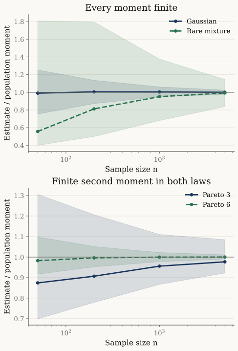
Independent repeated samples, 600 per law and sample size. Lines show medians; bands show the 10th–90th percentiles of the estimator divided by its population target. These are sampling-distribution summaries, not confidence bands for a fitted model or Monte Carlo confidence intervals. Every population second moment here is finite; Pareto with exponent 3 has an infinite fourth moment. The finite mixture also converges slowly on this grid, despite having every moment.
Fitting a model introduces another boundary¶
The known-cutoff Pareto plug-in uses .
Use pareto_mean_plugin.
from xmath.incerto.estimators import pareto_mean_plugin

for sample in ([1, 1], [1, 2], [4, 4]):
    print(f"{sample} {pareto_mean_plugin(sample, x_m=1):.4g}")
Output
[1, 1] 1
[1, 2] 1.53
[4, 4] inf
Under an exact iid Pareto model with , the log-excess average has a gamma density that is positive and continuous at 1. Consequently even conditional on a finite fit,
The linked note derives that density. Its positive lower bound on a small left neighborhood of 1 makes the expectation at least a positive multiple of . The squared estimator diverges there as well. A concentrated central part of a sampling distribution can coexist with divergent moments. Simulations must count non-finite fits; removing them does not remove the singularity of the remaining distribution. No universal ranking of the sample mean and this plug-in follows.
Rising power means and different targets¶
For fixed observations and positive weights summing to 1, define . For ,
We prove this with Jensen’s inequality for the strictly convex function on , then take a th root. Equality holds exactly when all are equal. The inequality also holds below 1; those expressions are not norms. At fixed positive weights, as : bound the weighted sum above by and below by at a maximizing coordinate .
For equal weights and observations , , , , and . The order changes which quantity is summarized; a larger value alone neither proves a power law nor diagnoses estimation failure.
For geometric unit balls, use the unnormalized norm . Its value decreases with at fixed . To prove this for , divide each coordinate by ; the resulting magnitudes are at most 1, so their th powers sum to at most their th powers, namely 1. The -unit balls therefore expand. In two dimensions, give a diamond, circle, and square, with areas 2, , and 4. The factor in explains why its monotonicity goes in the other direction.
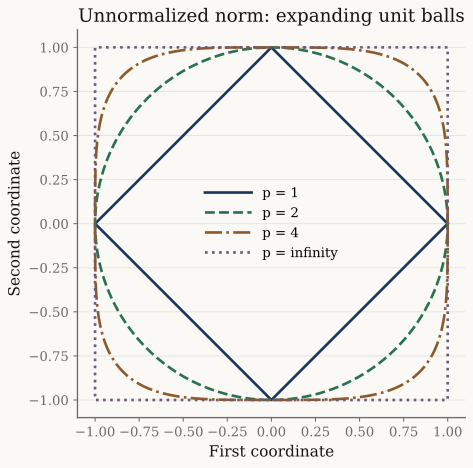
Exact geometric contours. These use the sum of powers, whereas the empirical power mean uses the average of powers. No probability model is needed for this comparison.
Mean absolute deviation is a different estimand¶
If and , then . If the variance is finite, Cauchy–Schwarz gives . Equality requires to be constant almost surely. These are unscaled deviations; Gaussian calibration multiplies the mean absolute deviation by , so that universal inequality does not apply to the calibrated value.
For example, the symmetric law on has standard deviation and unscaled mean absolute deviation both equal to 1. Its Gaussian-calibrated Std/MeanAD ratio is . The Gaussian benchmark 1 in the dispersion diagnostic is a model reference, not a universal lower bound. Mean and median absolute deviations also answer different questions. Neither universally replaces a second-moment estimand or dominates every estimator under every loss.
Reproduce and interpret¶
Use pareto_type1, pareto_moment_estimator_summary.
Code
import numpy as np
from xmath.incerto.distributions import pareto_type1
from xmath.incerto.finite_moments import pareto_moment_estimator_summary

rng = np.random.default_rng(20261020)
for alpha in (3, 6):
    sample = pareto_type1.rvs(alpha, size=(100, 200), random_state=rng)
    estimates = np.mean(sample**2, axis=1)
    print(f"alpha={alpha:.4g}")
    for name, value in pareto_moment_estimator_summary(alpha, q=2, n=200).items():
        print(f"  {name}: {value:.4g}")
    quantiles = np.quantile(estimates, [0.1, 0.5, 0.9])
    print("Sample quantiles: [" + ", ".join(f"{v:.4g}" for v in quantiles) + "]")
Output
alpha=3
  moment: 3
  estimator_variance: inf
Sample quantiles: [2.335, 2.726, 3.491]
alpha=6
  moment: 1.5
  estimator_variance: 0.00375
Sample quantiles: [1.433, 1.497, 1.592]
The quantiles describe 100 seeded second-moment estimates from samples of size 200.
Figure regeneration: uv run python demos/incerto/finite_moments.py. NumPy’s PCG64 generator
uses seed 20261018; sample sizes are 50, 200, 1000, and 5000, with 600
independent replications per law and size. The four laws are unit normal,
the stated rare-state mixture, and Pareto with , .
The script allocates one sample size at a time, about 3 million observations
at the largest size, and normally takes seconds. It performs no clipping,
censoring, external-data access, or silent non-finite removal.
The experiment illustrates finite-sample spread. The proofs above establish moment boundaries; a finite Monte Carlo variance cannot test an infinite population variance. Later chapters develop convergence rates and broader comparisons. The Cauchy running-statistics experiment belongs to chapter 7.
References¶
Taleb (2025), Statistical Consequences of Fat Tails, third edition, 2025, ch. 4, §§4.4–4.4.4, printed pp. 79–86, and §4.5, pp. 88–89: dispersion, moment estimation, and norm geometry. The precise estimator distinctions and proofs here are our own. The recommendation in §4.4.5, pp. 87–88 is not used as a universal statistical theorem.
The linked Pareto moment, infinite-mean, and plug-in notes supply the prerequisite proofs at their stated scopes.
- Taleb, N. N. (2025). Statistical Consequences of Fat Tails (3rd ed.). https://arxiv.org/abs/2001.10488v4