Dispersion Ratio Under Fat Tails

Statement¶

Let $x_1,\dots,x_n$ be observed data, and compare the sample standard deviation with absolute-deviation scale estimates. The repository uses normal-scaled versions

and

For Gaussian data, both are calibrated to estimate the same $\sigma$ as the standard deviation. Under fat-tailed or contaminated data, the ratios

can rise because sample standard deviation is more sensitive to isolated extremes. The mean absolute deviation uses all observations; the median absolute deviation depends on their central order statistics.

The sample notation $X_1,\dots,X_n$ and expectation notation follow the shared notation table. The scale symbol $\sigma$ and the names MeanAD and MedianAD are local conventions for this page.

Examples¶

• For Gaussian data, the standard deviation, normal-scaled mean absolute deviation, and normal-scaled median absolute deviation target the same $\sigma$, so the ratios should be near 1.

• For Student-t or Pareto samples, large observations can push the standard deviation much higher than the absolute-deviation scales.

Use dispersion_ratios.

from xmath.incerto.stats import dispersion_ratios

for sample in ([2, 2, 2], [0, 0, 10], [1, 2, 3]):
    mean_ratio, median_ratio = dispersion_ratios(sample)
    print(f"{sample}: Std/MeanAD={mean_ratio:.4g}, Std/MedianAD={median_ratio:.4g}")

Output

[2, 2, 2]: Std/MeanAD=nan, Std/MedianAD=nan
[0, 0, 10]: Std/MeanAD=0.8463, Std/MedianAD=inf
[1, 2, 3]: Std/MeanAD=0.9772, Std/MedianAD=0.5507

The ratios distinguish $0/0$ from a positive numerator over a zero denominator.

Calibration¶

We justify the Gaussian scale constants here; these identities do not establish a tail class. Integrating the standard normal density on the positive half-line gives $\mathbb E|Z|=2\int_0^\infty z\phi(z)\,dz=\sqrt{2/\pi}$. The equation $P(|Z|\le m)=2\Phi(m)-1=1/2$ gives $m=\Phi^{-1}(0.75)$. Here $Z$ is standard normal and $\phi$ is its density.

For $X\sim N(\mu,\sigma^2)$,

Thus multiplying the mean absolute deviation by $\sqrt{\pi/2}$ calibrates it to $\sigma$ under a normal model. Also,

so dividing the raw median absolute deviation by $\Phi^{-1}(0.75)$ gives the same normal calibration.

These identities are normal-model calibrations, not tail theorems. If the sample has extreme observations, the standard deviation’s quadratic loss gives those observations much more weight than either absolute-deviation statistic.

Simulation¶

The simulation compares Gaussian, Student-t, and Pareto samples across sample sizes. It reports repeated-simulation medians of the two dispersion ratios.

Use dispersion_ratios.

import numpy as np
from xmath.incerto.stats import dispersion_ratios

rng = np.random.default_rng(20261020)
for label, sample in (("Normal", rng.normal(size=5000)),
                      ("Student 3", rng.standard_t(3, size=5000))):
    values = dispersion_ratios(sample)
    print(f"{label}: [" + ", ".join(f"{v:.3f}" for v in values) + "]")

Output

Normal: [1.003, 1.021]
Student 3: [1.175, 1.383]

These are sample diagnostics, not estimates of a tail exponent.

Figure regeneration: uv run python demos/incerto/dispersion_ratio.py.

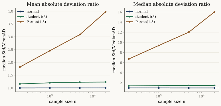
The Gaussian calibration explains why the simulated Gaussian ratios are near one. The Student-t and Pareto ratios are larger because the standard deviation is more sensitive to extremes than the absolute-deviation scales. The ratio is a stress signal, not a fitted tail exponent. The moment-estimation note explains why a finite population moment can still have an estimator with infinite variance.

Caveats¶

• A high ratio is a diagnostic, not a fitted tail exponent.

• The mean absolute deviation and median absolute deviation are scaled here to match a Gaussian standard deviation. Other conventions use unscaled values.

• Median absolute deviation can be too robust for payoff questions where a rare outlier dominates the quantity of interest.

• In an infinite-variance sample, the ratios are sample-path objects; the population variance does not exist.

• Dependence and volatility clustering can move these ratios even when the one-step marginal distribution is unchanged.

References¶

• Taleb (2025), Statistical Consequences of Fat Tails, third edition, 2025, ch. 4, §§4.4.1–4.4.3, printed pp. 79–84: dispersion comparisons. The Gaussian calibrations above are derived here.

• Rousseeuw & Croux (1993), “Alternatives to the Median Absolute Deviation”.

Backlinks¶

• Depends on: Variance Gamma Distribution and Body, Shoulders, and Tails.

• Used by: robust-scale examples and tail-risk diagnostics.

Recorded calculation¶

The committed demo produced the following on 2026-10-17. These are sample calculations, with seeds and sample sizes specified in the script.

normal; n=200; median Std/MeanAD=0.999; median Std/MedianAD=1.001
normal; n=1000; median Std/MeanAD=1.000; median Std/MedianAD=1.002
normal; n=5000; median Std/MeanAD=1.000; median Std/MedianAD=0.997
normal; n=20000; median Std/MeanAD=1.000; median Std/MedianAD=0.999
student-t(3); n=200; median Std/MeanAD=1.159; median Std/MedianAD=1.421
student-t(3); n=1000; median Std/MeanAD=1.202; median Std/MedianAD=1.464
student-t(3); n=5000; median Std/MeanAD=1.226; median Std/MedianAD=1.500
student-t(3); n=20000; median Std/MeanAD=1.231; median Std/MedianAD=1.497
Pareto(1.5); n=200; median Std/MeanAD=1.819; median Std/MedianAD=6.723
Pareto(1.5); n=1000; median Std/MeanAD=2.457; median Std/MedianAD=9.386
Pareto(1.5); n=5000; median Std/MeanAD=3.086; median Std/MedianAD=12.000
Pareto(1.5); n=20000; median Std/MeanAD=3.974; median Std/MedianAD=16.015