Pre-Asymptotic LLN Behavior

Setup¶

This synthetic example plots running means

for iid Pareto Type I samples with $x_m=1$. The target contrast is:

• if $\alpha\le1$, LLN Failure Under Infinite Mean says $\bar X_n\to\infty$ almost surely;

• if $\alpha>1$, the finite-mean law of large numbers says $\bar X_n\to\alpha/(\alpha-1)$, but convergence can still be slow when $\alpha$ is close to 1.

The symbols $\bar X_n$, $S_n$, $\alpha$, and $x_m$ follow the shared notation table.

What the simulation isolates¶

The simulation uses exact iid Pareto draws. It does not include dependence, threshold fitting, censoring, mixtures, or measurement error. That narrow setup is deliberate: it isolates why the theorem can be practically easy to underestimate even before empirical complications enter.

The inverse-transform representation is

The distribution helper in xmath.incerto.distributions implements the same Pareto Type I law.

Running-mean paths¶

The left panel shows single running-mean paths at log-spaced checkpoints. The right panel summarizes repeated final sample means at several sample sizes.

Use pareto_type1, running_mean, max_to_sum_ratio.

import numpy as np
from xmath.incerto.distributions import pareto_type1
from xmath.incerto.estimators import running_mean, max_to_sum_ratio

rng = np.random.default_rng(20261020)
for alpha in (0.8, 1.0, 1.3):
    sample = pareto_type1.rvs(alpha, size=5000, random_state=rng)
    means = running_mean(sample)[[99, 999, 4999]]
    print(f"alpha={alpha:.4g}: [" + ", ".join(f"{v:.4g}" for v in means) + "]")
    print(f"Maximum share: {max_to_sum_ratio(sample):.3f}")

Output

alpha=0.8: [127, 81.28, 37.8]
Maximum share: 0.115
alpha=1: [5.203, 7.27, 8.461]
Maximum share: 0.064
alpha=1.3: [3.292, 5.847, 4.178]
Maximum share: 0.097

Only the $\alpha=1.3$ law has a finite population mean, $13/3$; a finite path does not prove convergence.

Figure regeneration: uv run python demos/incerto/lln_preasymptotic.py.

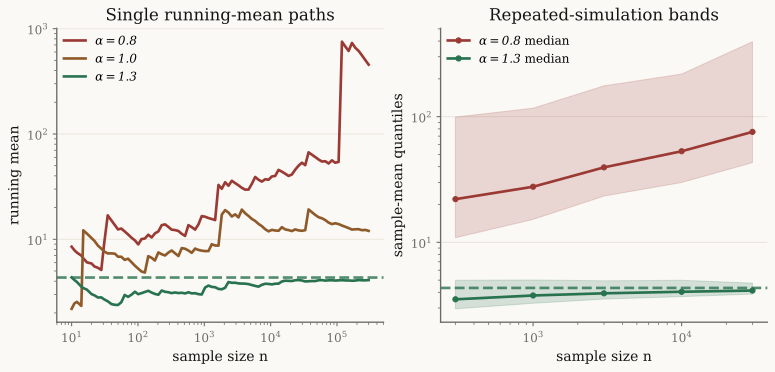
For $\alpha\le1$, no finite theoretical mean exists. For $\alpha=1.3$, the finite mean exists, but large observations still create visible pre-asymptotic jumps and wide repeated-simulation bands.

Interpretation and caveats¶

• One simulated path is not a proof and not an estimator of $\alpha$.

• The plot uses log axes. This makes early and late behavior comparable, but it also visually compresses large jumps.

• A path with $\alpha>1$ can look worse than a path with $\alpha\le1$ over a finite window if it happens to receive an unusually large early draw.

• Real data adds threshold choice, dependence, measurement limits, and model uncertainty. The example isolates only the iid Pareto mechanism.

References¶

• Feller (1971), An Introduction to Probability Theory and Its Applications, Vol. II.

• Resnick (2007), Heavy-Tail Phenomena.

Backlinks¶

• Depends on: Pareto Distribution and LLN Failure Under Infinite Mean.

• Used by: Max-to-Sum Ratio and Generalized Central Limit Theorem.

Recorded calculation¶

The committed demo produced the following on 2026-10-17. These are sample calculations, with seeds and sample sizes specified in the script.

Pareto alpha=0.8:
  final running mean after 300,000 draws: 454.983
  largest observation's share of total: 0.600
  finite theoretical mean: none
Pareto alpha=1.0:
  final running mean after 300,000 draws: 12.020
  largest observation's share of total: 0.070
  finite theoretical mean: none
Pareto alpha=1.3:
  final running mean after 300,000 draws: 4.100
  largest observation's share of total: 0.010
  finite theoretical mean: 4.333