Are NYC Dog Names Fat-Tailed?

Setup¶

Cook (2026), in “Dogs and fat tails”, studies the distribution of dog-name frequencies. Bella and Luna have plenty of company, while thousands of names appear only once. A lognormal describes the overall pattern reasonably well. Here we draw the rank-frequency picture too, then examine how tail estimates change across thresholds.

The source is the NYC Dog Licensing Dataset New York City Department of Health and Mental Hygiene, 2026. Each source row is an active license period, not necessarily a unique dog. A renewal within the same year can add another row for the same animal. We therefore call the aggregated values license-period frequencies, not dog counts.

We use the full public dataset, not a little row sample. The Socrata API does the compacting for us: trim and uppercase the names, drop missing-name placeholders, and return one count per name. The result is only about 35,000 rows instead of hundreds of thousands of license records, so the complete aggregate is small enough to travel with the page.

What is being estimated?¶

Let $x_i$ be the number of included license-period records attached to the $i$th observed normalized name. The sample for the tail diagnostics is

where $n$ is the number of distinct names in the snapshot. A large $x_i$ means that a name is popular. Names that do not occur in the licensing data are absent, so this is a zero-truncated frequency spectrum rather than a sample of all possible names.

A whole-sample lognormal fit and a tail estimate answer different questions. The first summarizes all positive frequencies. The second requires a high threshold and asks whether the observations above it behave approximately like a regularly varying right tail. We use the Hill estimator and a generalized Pareto shape fit across many candidate thresholds, following Tail Threshold Selection. No body/shoulder boundary supplies that threshold automatically.

First, the dog-name popularity curve¶

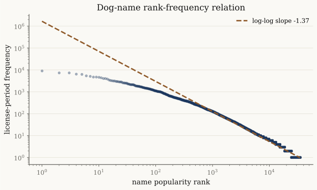
Sort names from most to least frequent, give them ranks $1,2,\ldots,n$, and plot rank against frequency. A power law would look roughly straight on log-log axes. The dashed line is an ordinary least-squares fit in log space; it is a visual summary, not a claim that dog naming follows an exact law.

Global fit and threshold sensitivity¶

The survival plot compares the data with the blog’s global lognormal baseline. Below it, two roomier panels use only upper frequencies and expose the threshold choice. The generalized Pareto fit uses the GPD shape parameter $\xi$; the Hill panel reports the Pareto tail exponent $\widehat\alpha=1/\widehat\xi$. These symbols follow the shared notation table.

Use load_nyc_dog_name_frequencies, hill_stability, DogNameFrequencyData.frequency_for.

from xmath.incerto.datasets import load_nyc_dog_name_frequencies
from xmath.incerto.estimators import hill_stability

data = load_nyc_dog_name_frequencies()
print(f"Names / records: {data.name.size:d} {data.frequency.sum():d}")
print(f"Safari: {data.frequency_for('Safari'):d}")
result = hill_stability(data.frequency, [50, 200, 1000])
print("Hill alpha: [" + ", ".join(f"{v:.3f}" for v in result["alpha"]) + "]")

Output

Names / records: 34680 789724
Safari: 3
Hill alpha: [1.896, 1.287, 1.056]

The bundled aggregate is read locally in an editable checkout.

Figure regeneration: uv run python demos/incerto/nyc_dog_name_tail.py.

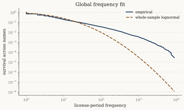
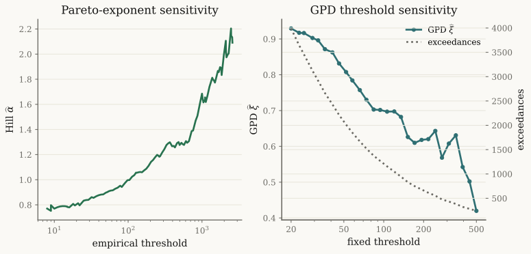
The survival view adds a finding beyond the global distribution label: the empirical far-right curve lies above the whole-sample lognormal fit. The tail panels then show that this extra upper-tail mass does not settle into a broad, flat Hill region. The GPD shape estimate also falls as the threshold rises while the number of exceedances shrinks. The data therefore do not support reporting one threshold-insensitive Pareto exponent.

This does not establish a lognormal data-generating mechanism. It says that, within the observed pooled snapshot, the upper frequencies do not give stable evidence for one Pareto-type tail. A lognormal or another non-Pareto model can mimic a power law over a finite range, and the current sample does not settle the asymptotic class.

A name lookup¶

The same aggregate can answer case-insensitive name-frequency questions. The result remains a count of license-period rows unless the underlying records can be shown to represent different dogs.

Use load_nyc_dog_name_frequencies, DogNameFrequencyData.frequency_for.

from xmath.incerto.datasets import load_nyc_dog_name_frequencies

data = load_nyc_dog_name_frequencies()
for name in ("Safari", " safari ", "SAFARI"):
    print(f"{name!r}: {data.frequency_for(name):d}")

Output

'Safari': 3
' safari ': 3
'SAFARI': 3

Caveats¶

• The source counts license periods. Renewals can cause multiple rows for one dog, and the public columns do not contain a stable dog identifier.

• The dataset pools extract years. It mixes changing name preferences, population turnover, and repeated licensing periods.

• Uppercasing and trimming do not merge spelling, punctuation, or transcription variants.

• Frequencies are discrete, tied, and dependent because they sum to the total number of included records. The iid continuous-tail assumptions behind Hill and GPD asymptotics are therefore approximations here.

• Only observed names enter the sample. Unused possible names have zero frequency and are not represented.

• Threshold stability is an empirical diagnostic, not a proof of a tail class. A larger or differently deduplicated sample could give a different pattern.

References¶

• Cook (2026), “Dogs and fat tails”.

• New York City Department of Health and Mental Hygiene (2026), “NYC Dog Licensing Dataset”.

• Taleb (2020), Statistical Consequences of Fat Tails.

• Hill (1975), “A Simple General Approach to Inference About the Tail of a Distribution”.

• Coles (2001), An Introduction to Statistical Modeling of Extreme Values.

Backlinks¶

• Depends on: Hill Estimator, Tail Threshold Selection, and the Generalized Pareto Distribution.

• Related: Body, Shoulders, and Tails describes variance-mixture density geometry; it is not an empirical tail threshold rule.

• Related empirical work: Amazon Book Rank Tail Diagnostics.

Recorded calculation¶

The committed demo produced the following on 2026-10-17. These are sample calculations, with seeds and sample sizes specified in the script.

NYC dog-name frequencies
  Normalized names: 34,680
  Included license-period records: 789,724
  Largest name frequency: 8,899
  Rank-frequency log-log slope: -1.372 (R^2=0.977)
  Whole-sample lognormal parameters: shape=1.387, scale=3.858

Selected tail-sensitivity points
  k=   50; threshold=  1758; Hill alpha=1.896
  k=  100; threshold=  1100; Hill alpha=1.639
  k=  200; threshold=   581; Hill alpha=1.287
  k=  500; threshold=   264; Hill alpha=1.183
  k=1,000; threshold=   128; Hill alpha=1.056
  k=2,000; threshold=    53; Hill alpha=0.903
  k=5,000; threshold=    15; Hill alpha=0.783
Safari: 3 included license-period records