A Gaussian conditional model need not give a Gaussian marginal law. Let and let be independent of . We study
Here is variance, so is conditional standard deviation. This is the centered scalar case of the Normix normal-mixture construction. We use its shared mixing symbol and the notation canon. A one-observation mixture specifies no temporal dependence: volatility clustering requires a model for a sequence of mixing variables.
Which moments does mixing preserve?¶
For every real , the absolute moment factors, including infinite values:
We prove this identity by independence and Tonelli’s theorem applied to the nonnegative product . In the normal integral for , the substitution gives the displayed gamma integral. Thus the moment exists exactly when the mixing moment exists. Symmetry alone does not make an odd signed moment exist; absolute integrability is still required.
If , then , and . If also , its Pearson kurtosis is
The Gaussian reference is 3. For fixed mean variance, nonconstant raises kurtosis. This comparison is specific to centered normal variance mixtures; it is not an ordering of arbitrary distributions by tail risk.
Two states, finite moments¶
Choose equal probabilities for and , with . Conditioning gives variance 1 and fourth moment . At these are 1 and 4.08. The density is the average of two Gaussian densities. Its moment generating function (MGF) and characteristic function are
They follow from the two conditional Gaussian transforms. They are different functions, even though the mean is zero. For , division by the unit-normal density gives
The narrower component’s ratio tends to zero; the wider component’s ratio increases without bound. Nevertheless is finite for every real . The mixture has more far-tail density than the unit normal and still satisfies the Cramér condition. It is not a power law. At the lower state is an atom at zero and the full law no longer has a Lebesgue density.
Unequal probabilities remove the equal-weight example’s kurtosis ceiling. For a different worked case, take
Then , and kurtosis is 77.25. All moments and the MGF remain finite. More generally, fixing and putting probability on and on preserves , while diverges as . Each fixed still gives a finite Gaussian mixture. A rare state can make a finite moment hard to estimate without making it infinite.
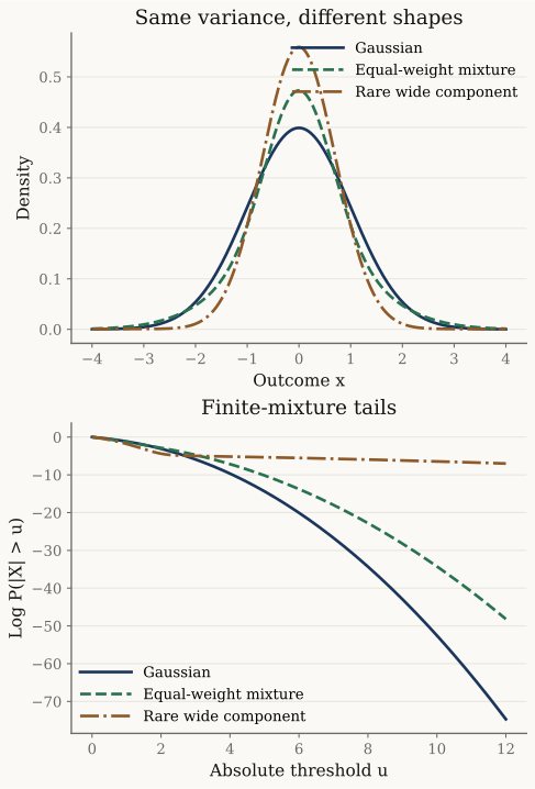
Exact mixture densities and two-sided probabilities. All three laws have variance 1. The rare wide component is visible in the survival plot even where its contribution to central density is small. No samples or data fits are used.
Variance and precision give different laws¶
Three explicit constructions show why the distribution of the mixing variable matters. All parameters below are local to this section.
Gamma variance. Let have gamma shape and scale , so . Integrating its density gives
For the MGF, condition on and integrate against the gamma density. The integral diverges at and beyond the endpoints. All positive power moments exist, and kurtosis is . At , the MGF is that of a centered Laplace law with scale ; this law has exponential tails. The density calculation below gives the general gamma-mixture decay.
Lognormal variance. Let , where is standard normal, independent of , and . Completing the square gives
Every positive power moment exists, yet for every . To see divergence, write the expectation as an integral over ; its exponent contains a positive multiple of minus , and is eventually positive on an infinite half-line. Finite moments of every order therefore do not imply a finite MGF. Nor does this construction have a finite power-tail exponent: a regularly varying survival with finite positive exponent would force sufficiently high moments to diverge.
Gamma precision. Let have gamma shape and rate , with . Integrating the conditional density gives
Indeed the integrand is proportional to , a gamma integral. This is Student’s law at unit scale. Its density is asymptotic to a positive constant times ; integrating that comparison gives a survival exponent . The moment identity above reduces to an integral of near zero for moment order , so exactly when . For its variance is , not 1.
These are proved model calculations. SCoFT v4 §4.2, pp. 74–75 supplies the variance-versus-precision question; it is not a claim that every stochastic volatility model produces a power law. Recursive uncertainty belongs to a later treatment and requires a specified limiting construction.
Reproduce the worked cases¶
Use normal_mixture_absolute_moment, normal_mixture_log_abs_survival.
import numpy as np
from xmath.incerto.finite_moments import (
    normal_mixture_absolute_moment, normal_mixture_log_abs_survival,
)

for variances, weights in (([1], [1]), ([0.5, 50.5], [0.99, 0.01])):
    m2 = normal_mixture_absolute_moment(2, variances, weights)
    m4 = normal_mixture_absolute_moment(4, variances, weights)
    tail = np.exp(normal_mixture_log_abs_survival(4, variances, weights))
    print(f"Variance / kurtosis / P(|X|>4): {m2:.4g} {m4 / m2**2:.4g} {tail:.4g}")
Output
Variance / kurtosis / P(|X|>4): 1 3 6.334e-05
Variance / kurtosis / P(|X|>4): 1 77.25 0.005735
All moments of these two finite Gaussian mixtures exist.
Figure regeneration: uv run python demos/incerto/finite_moments.py. The mixture curves use
801 central-density and 241 tail-threshold points, with the parameters above.
The script also checks moment formulas and reports a bounded, seeded
estimation experiment described in moment estimation.
Body and shoulder geometry explains which
parts of a density gain or lose under a small variance perturbation.
Variance–mean gamma calculation¶
The following extension permits a moving conditional mean.
For a gamma mixture, let
(shape and scale) and . The local parameters satisfy
, , and .
The helper univariate_variance_gamma(alpha, beta, lam) uses
alpha for , beta for , and lam for ; its alpha
is not the Pareto exponent. Conditioning and the gamma MGF give
The interval follows by solving the positive-quadratic-base inequality. The variance follows from conditional variance plus the variance of the conditional mean. For , integrating the conditional Gaussian density against the gamma density gives
To obtain this expression, substitute , , in the Bessel integral for . The standard Bessel asymptotic then gives right and left density decay rates and , each with a power factor . These are exponential tails, not regularly varying ones. The integral representation and special-function asymptotics are used as standard identities, not proved here DLMF 10.32.10 and DLMF 10.40.2.
At the origin, the same density integral is a gamma integral when , giving
For smaller shapes it diverges: the Bessel limits give a logarithmic singularity at and an integrable power singularity below it. Here the small-argument Bessel limits are cited from DLMF 10.30.2–3. The symmetric case , reduces to the Laplace density . The general family relationships remain in the Normix family tour.
References¶
Taleb (2025), Statistical Consequences of Fat Tails, third edition, 2025, ch. 4, §§4.1–4.2, printed pp. 69–75: mixture mechanisms. The calculations above state their own hypotheses and proofs.
The linked DLMF identities supply the Bessel integral and asymptotics used only in the variance–mean gamma density calculation.
- Taleb, N. N. (2025). Statistical Consequences of Fat Tails (3rd ed.). https://arxiv.org/abs/2001.10488v4