The speed of a uniformly sampled particle in a two-dimensional equilibrium gas has a Rayleigh distribution. Each signed velocity component is Gaussian; taking the length of the velocity vector changes the law. This answers Taleb’s distribution challenge Taleb, 2026: the density already written in the accompanying animation is Rayleigh Matharium, 2026. No extra physical parameter is needed.
The sampling rule matters. An event recorded when a particle crosses a small hole favors faster particles. We derive the chamber law first, then the effusion law and the finite-system correction. A seeded simulation compares seven fitted families; it illustrates these distinctions without testing whether the animation implements equilibrium dynamics.
From components to speed¶
Assume a classical, nonrelativistic gas of equal-mass particles at canonical equilibrium, with no bulk flow and no constraint on total momentum. Let be particle mass, temperature, and Boltzmann’s constant. Let be an integer. Write the velocity as , the speed as , and its realized value as . Set
Here is component standard deviation; it is not speed standard deviation. Densities below use Lebesgue measure in their stated coordinates. These symbols agree with the shared notation.
For particles at positions and a velocity-independent potential , the Hamiltonian is , and the canonical weight separates into kinetic and positional factors Tong, n.d., §2.3. Integrating the positions and the other particles leaves the single-particle density
The factorization proves that the components are independent variables. This follows from the equilibrium measure; it does not require a central limit argument about collisions. The maximum-entropy note explains why the constraint and the coordinate measure must be specified in an entropy argument.
We now derive the speed density, its moments, and its mode. The surface area of the unit sphere in dimensions is . Polar coordinates contribute the shell factor , giving
The density is zero for , and . Substitution gives
Taking proves normalization. For every real ,
For the integral diverges at zero. Every positive moment exists. For , differentiating the log density gives , so the unique mode is . For the law is half-normal and its mode is zero.
| Dimension | Law and density for | Mean | Variance | Mode |
|---|---|---|---|---|
| 2 | Rayleigh: | |||
| 3 | Maxwell: |
In two dimensions, integration also gives for . This is a Weibull law with shape 2 and scale . Its right tail decays faster than any exponential, placing it on the light side of the tail-class catalog.
Generalized Gamma, not GIG¶
For a local shape , define
This is a generalized Gamma density with power 2; the chamber law has . The generalized inverse Gaussian GIG family is a different family. In the shared convention its kernel is , with and .
We can exclude Gamma, inverse Gamma, inverse Gaussian, and GIG by their tails, without fitting any data. In the following kernels, shapes and scales are positive, and all parameters are fixed as .
| Candidate | Density kernel on |
|---|---|
| Gamma, shape , scale | |
| Inverse Gamma, shape , scale | |
| Inverse Gaussian, mean , shape | |
After taking logarithms, each candidate has only constant, logarithmic, linear, and reciprocal terms. Consequently, for each such density ,
The unequal limits prove that none of these fixed-parameter laws equals . The argument includes the normalizable Gamma and inverse Gamma boundaries of GIG. Log densities refer to a fixed choice of speed units; changing units changes the negative constant but preserves the distinction.
Gaussian exclusion needs a separate argument: a nondegenerate Gaussian assigns positive probability to negative speeds. Its log-density limit is also negative, so the preceding tail test alone would not exclude it. For , even an ordinary Gaussian conditioned to be nonnegative fails: its density has a positive right limit at zero, whereas . Positive support and skewness alone do not identify a family.
Squared speed and energy¶
Let and let be kinetic energy. The change of variable from to has Jacobian , so under ,
Using Gamma’s shape, scale convention, this proves
For the 2D chamber, : squared speed is exponential with mean , and kinetic energy is exponential with mean . For , a second Jacobian gives
Thus . Similarly has inverse Gamma scale . The reciprocal speed instead has an exponential factor ; it is not inverse Gamma.
If the normalizable boundaries are included, and . For the strict family these are limits. Transforming a Gamma variable by a square root does not preserve membership in Gamma or GIG.
Crossing a hole changes the sample¶
Assume the hole is small compared with the mean free path, the gas near it is isotropic and equilibrated, and detection efficiency does not depend on speed. In time , particles that can cross a small area come from a layer of thickness , where is the angle to the outward normal and . This is the flux factor in the usual effusion calculation Fitzpatrick, n.d..
Multiplying the equilibrium velocity measure by this factor and integrating over outward directions leaves one extra factor . Normalizing proves
The effusing speed divided by therefore has law . In particular,
Two-dimensional effusion has the same speed law as a three-dimensional chamber. The change comes from sampling, not an added spatial dimension. Its mode is , and its squared speed and energy use in the preceding Gamma formulas. Selecting only an outward direction would not introduce the factor ; counting crossings does.
The animation shows particles leaving an opening and accumulating in a histogram Matharium, 2026. If those are physical crossing events, the effusion law is the appropriate equilibrium prediction. If the opening merely conveys uniformly selected particles to a histogram, Rayleigh is appropriate. The displayed formula specifies the chamber law; without the sampling algorithm, the drawing does not resolve this distinction.
A finite isolated chamber¶
Canonical velocities have the preceding Gaussian components even for finite . An isolated finite system with fixed total kinetic energy has a different joint measure. Assume ideal particles, or elastic hard disks or spheres, in reflecting hard walls, with total kinetic energy and no imposed total-momentum constraint. The velocity measure is uniform on the sphere
We derive its one-particle marginal. Integrating the remaining coordinates against the energy-shell delta function supplies the factor . The first particle’s radial element contributes . Put and . Substitution normalizes the density to
Equivalently,
This is a scaled Beta energy law, with a finite upper endpoint Scalas et al., 2015. For the instantaneous effusion measure, multiplication by changes the first Beta shape to , leaving the second unchanged.
Define the kinetic temperature by . At fixed and fixed speed, the finite-system factor tends to as , and the Gamma-ratio asymptotic gives the canonical normalizer. This proves the chi limit; it is not a uniform relative approximation all the way to . Fixing total momentum as well would change the available degrees of freedom and the Beta law.
Hard-core exclusion affects the allowed positions but introduces no velocity-dependent potential, so it does not alter the canonical factorization. Elastic collisions conserve energy; that alone does not prove that an arbitrary initial condition has equilibrated. Noninteracting point particles reflecting in a fixed box retain their individual speeds.
Leaking cools the chamber¶
The moment formula gives mean energy inside and among effusing particles. A leak therefore removes more energy per particle than the chamber average. In a large, unheated chamber that re-equilibrates between losses, treat as continuous and use dots for time derivatives. Energy balance gives
Since , temperature falls. Starting at , integration gives within this quasistatic approximation. If the outgoing event rate is , the accumulated speed density over an observation interval is
It generally mixes temperatures. The variance-mixture note explains why averaging over scales can change a marginal law. A fixed-temperature effusion density does not describe an entire cooling history.
A reproducible comparison¶
We draw 50,000 independent pairs of Gaussian components with , seed 20261022, and take their Euclidean lengths. All first components are drawn before all second components. This samples the canonical chamber law directly; it is neither molecular dynamics nor a sample extracted from the animation.
We fit Gaussian, Gamma, inverse Gamma, inverse Gaussian, GIG, Rayleigh, and Weibull laws by maximum likelihood. Positive families have location fixed at zero. Gaussian estimates mean and standard deviation; Rayleigh estimates one scale; Weibull, Gamma, and the two inverse families estimate two parameters. With estimated parameters and maximized log likelihood , the reported score is in these fixed speed units.
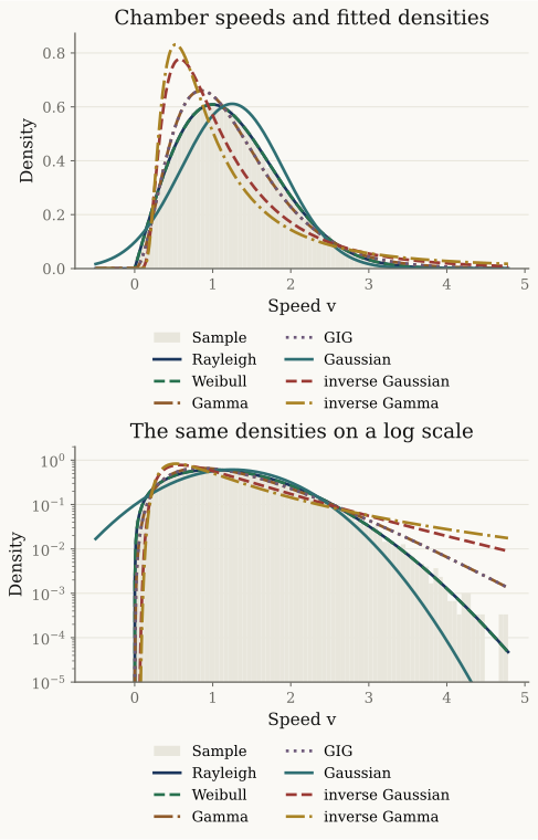
The same 50,000 speeds in 80 bins. Curves use 401 points from -0.5 to the sample maximum. The log panel displays densities down to 10-5; this plotting limit does not truncate the fitted laws. Rayleigh and Weibull nearly coincide, as do Gamma and the GIG boundary fit.
The table’s KS distance is , where is the empirical CDF. Its p-values are the ordinary two-sided KS calculation without correction for parameter fitting. They are descriptive diagnostics, not calibrated tests of the fitted families. Calibration would require, for example, a parametric bootstrap with refitting in each replicate SciPy developers, 2026. Zeros below are numerical underflow, not exact zero probabilities.
Use sample_chi_speed,
fit_speed_models,
speed_fit_table, and
squared_speed_ks.
Code and fit table
from xmath.incerto.gas_speeds import (
    sample_chi_speed, fit_speed_models, speed_fit_table, squared_speed_ks,
)

v = sample_chi_speed(50_000, random_state=20261022)
fits = fit_speed_models(v)
print(speed_fit_table(fits))
energy = squared_speed_ks(v, thermal_variance=1)
print(f"V^2 vs Exp(mean 2): D={energy['statistic']:.4f}, p={energy['pvalue']:.4f}")
for fit in fits:
    if fit.boundary:
        print(f"{fit.name} boundary: {fit.boundary}")
Output
Model              K        AIC     KS D   KS p (raw)
Rayleigh           1    93781.3   0.0034        0.618
Weibull            2    93783.3   0.0035        0.585
Gamma              2    95323.5   0.0327     5.43e-47
GIG                3    95325.5   0.0327     5.43e-47
Gaussian           2    99241.9   0.0471     5.06e-97
inverse Gaussian   2   110562.7   0.1170            0
inverse Gamma      2   123078.8   0.1338            0
V^2 vs Exp(mean 2): D=0.0058, p=0.0696
GIG boundary: Gamma
The Rayleigh scale estimate is about 0.9967. Weibull estimates shape 2.0014, close to Rayleigh’s exact shape 2; its extra parameter raises AIC by about 2. These are finite-sample fits, not a new derivation of the law.
Why the GIG fit lands on Gamma¶
The Gamma MLE has shape and scale . At its GIG representation , the inward derivative of log likelihood per observation is
This expression is finite because . Differentiating the normalizing integral supplies the model reciprocal mean in the first term. The other two score components vanish at the Gamma MLE. Log likelihood is concave in the natural coordinates : the Hessian of its log normalizer is the covariance of in the interior. The supporting-plane inequality therefore certifies a maximum on the Gamma boundary. For strict , this value is a supremum as .
The helper uses that boundary law directly for its density and CDF. It does not present tiny positive GIG parameters as a distinct distribution. The table retains GIG’s nominal , hence a score exactly 2 above Gamma’s. Ordinary regular-model AIC theory does not apply unchanged at this boundary; the score here is a stated comparison convention.
Quantiles and the squared-speed check¶
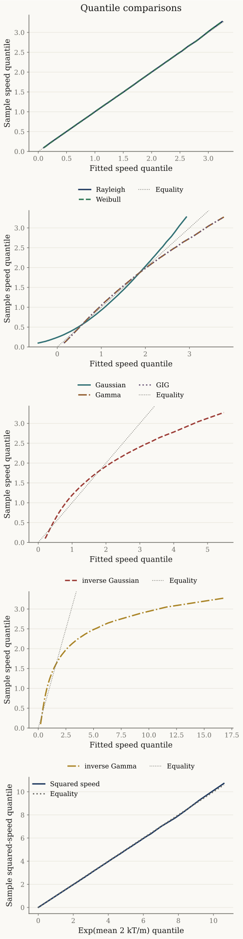
Theoretical quantiles are horizontal and empirical quantiles vertical, at 199 equally spaced probabilities from 0.005 to 0.995. The inverse-family panels need different horizontal ranges because their predicted upper quantiles are much larger. All displayed quantiles are retained. These QQ plots use the same observations as the fit table; they are not independent validation data.
The squared-speed test compares against the specified exponential mean 2, without estimating it. Its KS statistic is 0.0058 and its p-value is 0.0696, so it does not reject this simple null at the 5% level. This p-value has the usual iid continuous-null calibration. It is not the probability that the exponential model is true. The different Rayleigh p-value in the table uses a fitted scale.
chi_speed provides the model
density and CDF; speed_qq constructs
quantile pairs. The two figures come from
speed_fit_figure, using the
shared set_theme,
vertical_figure, and
savefig helpers.
Regenerate them with uv run python demos/incerto/rayleigh_speed.py.
The page’s text output is regenerated by
uv run python scripts/regenerate_incerto_outputs.py.
References¶
Taleb (2026) and Matharium (2026): the challenge and animation.
Tong (n.d.), §2.3: canonical velocity and Maxwell speed laws.
Fitzpatrick (n.d.): weighting wall crossings by normal velocity.
Scalas et al. (2015): finite microcanonical velocity and energy laws, including how boundary conditions change the constraints.
SciPy developers (2026): goodness-of-fit calibration with estimated parameters.
Browse the distribution catalog for related laws and the API reference for the reproducible calculations.
- Taleb, N. N. (2026). A challenge about the distribution of gas speeds. X post, 22 October. https://x.com/nntaleb/status/2113276779041345936
- Matharium. (2026). Two-dimensional Maxwell–Boltzmann speed animation. X post, 22 October. https://x.com/matharium/status/2113194382883197403
- Tong, D. (n.d.). Statistical Physics: Classical Gases. University of Cambridge lecture notes, section 2.3. https://www.damtp.cam.ac.uk/user/tong/statphys/statmechhtml/S2.html
- Fitzpatrick, R. (n.d.). Effusion. University of Texas at Austin thermal physics notes. https://farside.ph.utexas.edu/teaching/sm1/Thermalhtml/node88.html
- Scalas, E., Gabriel, A. T., Martin, E., & Germano, G. (2015). Velocity and Energy Distributions in Microcanonical Ensembles of Hard Spheres. Physical Review E, 92(2), 022140. https://arxiv.org/abs/1207.3505v2
- SciPy developers. (2026). scipy.stats.goodness_of_fit. SciPy API reference. https://docs.scipy.org/doc/scipy/reference/generated/scipy.stats.goodness_of_fit.html