An entropy maximizer answers a constrained optimization question. Specifying only “maximum entropy” leaves that question incomplete: the support, measure, and constraints determine the answer. Here all densities are with respect to Lebesgue measure in the stated coordinate, with natural logarithms and fixed measurement units.
Appendix B of Taleb (2025), printed pp. 127–133, motivates the examples. We prove the Shannon optima below by a relative-entropy bound. We then derive the normalization and moments of a q-exponential family and distinguish them from a global optimization theorem under escort constraints.
A certificate for a Shannon maximum¶
For a density on a fixed support , its differential entropy is , when defined. Consider a candidate
with finite normalizer and prescribed expectations of the sufficient statistics . This is the exponential-family form; , , and follow the shared notation. Assume the candidate and competitors have the same finite constraints, and .
We prove the entropy bound and its equality condition. With , for , with equality only at . Integrating against gives
Because is affine in the constrained statistics, . Consequently
This identity also permits and infinite KL when the cross entropy is finite. The negative part of is integrable against , so the right side is well-defined. Equality requires almost everywhere. This proves a global maximum, once a feasible candidate exists. It does not assert existence for arbitrary moment constraints.
Uniform and Gaussian constraints¶
On with finite , normalization alone gives and . Its log density is constant, so the certificate applies to every competing density on that interval. There is no corresponding uniform probability density on the whole real line.
On , fix and . The Gaussian candidate has
Its normalization is the Gaussian integral, and taking the prescribed second moment gives the displayed entropy. The certificate proves its unique maximum among densities with those moments. A half-line support would be a different optimization problem. These are the scoped versions of the examples in §B.1.1 and §B.1.3, pp. 128–129.
A logarithmic constraint selects Pareto¶
Fix , support , and
Here is a local log-moment, not . Put . The Pareto candidate is . To check feasibility, set ; its transformed density is on . Thus . Also
The entropy certificate proves that this Pareto law is the unique maximum for the stated log-moment constraint. No ordinary mean is required: it is finite only when , by the moment theorem. This supplies a complete proof for the model considered in §B.1.2, p. 129.
The constraint uses a dimensionless logarithm. Changing units from to changes entropy by and changes by the same factor. More generally, a differentiable increasing coordinate change with positive derivative gives whenever the terms are finite, by substitution in the density integral. A nonlinear change of coordinates therefore need not preserve an entropy ranking. For the logarithm above the correction is fixed by the constraint, which is why maximizing in either coordinate gives the same candidate here.
Tsallis entropy and escort constraints¶
For a local parameter , , define
provided . The second expression is an escort density. Its mean is a different functional from . Differential densities can exceed one, so inequalities between and require the value of , as well as the sign of .
For independent variables with densities and finite integrals of their th powers, Tonelli gives . Substitution proves
This concerns the joint density of the pair. It is not an entropy identity for the distribution of their sum. Since differential entropies can be negative, a universal superadditive/subadditive label needs further conditions. This distinction matters in §B.2, pp. 129–130.
To see where the family in that section comes from, write and prescribe an escort mean . For admissible variations at a positive density, differentiation of the numerator and denominator gives
A stationary density for subject to normalization and that constraint therefore satisfies, for Lagrange multipliers ,
This is a necessary interior stationarity calculation, with variations for which differentiation under the integral is justified. On an admissible branch it produces a power of an affine function. The escort constraint is nonlinear in ; we do not infer a global maximum from this calculation.
Normalize before interpreting the q-exponential¶
Take . The following family is a probability density for :
For its support is ; for it is , with density zero beyond that endpoint. At define for . We now prove normalization, the tail exponent, and the mean distinctions.
Substitution gives an unnormalized integral in both ranges. On the infinite support it converges only for ; diverges logarithmically and also fails. The survival on the interior of the support is
For , this is a Lomax survival with and scale . The same power comparison as in the Pareto moment proof shows exactly when ; equality diverges. All nonnegative power moments exist in the compact-support case. Integrating this survival gives
The ordinary mean is infinite for . In contrast, dividing by its integral gives a density proportional to . Integration gives
These formulas also have the stated exponential values at by limits. For and , the survival exponent is 3, ordinary mean is 1, and escort mean is . A zero escort mean on would force the escort law to concentrate at zero, impossible for this nondegenerate density. Centering a coordinate shifts the support too; it cannot set that mean to zero while preserving the same half-line. These restrictions qualify the normalization step in §B.2, pp. 132–133.
A worked comparison at fixed log-moment¶
Set , . In the coordinate , the maximizer is exponential with rate 2. A competitor with the same mean is gamma with shape 2 and rate 4, density on . Transforming back gives a log-gamma density for . Both meet the log-moment constraint, but their ordinary means differ: 2 for the Pareto and for the competitor.
Numerical integration of the log-coordinate entropy plus the Jacobian correction gives entropies approximately 0.806853 and 0.690921. Their gap, 0.115932, agrees with direct integration of and is positive as the certificate requires. Both calculations integrate to infinity; plotting endpoints do not truncate either model.
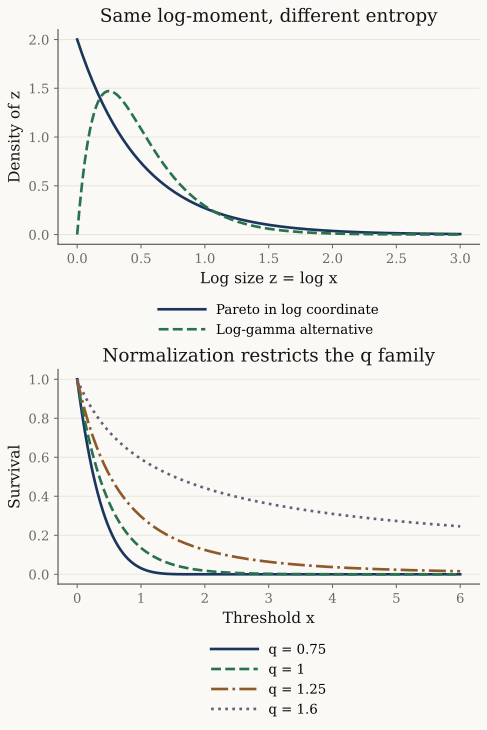
Top: exact log-coordinate densities with mean . Bottom: exact survival functions at , for . The compact-support survival reaches zero at 2 and stays zero. The other laws retain infinite support; the plotted range is finite. These are model calculations, with no sampled or observed data.
Use entropy_log_constraint_example.
from xmath.incerto.power_laws import entropy_log_constraint_example

result = entropy_log_constraint_example()
for name, value in result.items():
    print(f"{name}: {value:.4g}")
Output
pareto_mass: 1
pareto_log_moment: 0.5
pareto_entropy: 0.8069
log_gamma_mass: 1
log_gamma_log_moment: 0.5
log_gamma_entropy: 0.6909
kl: 0.1159
This quadrature checks one worked case, not global optimality.
Figure regeneration: uv run python demos/incerto/power_laws.py. The helper checks the
constraint, entropy and KL integrals independently by adaptive quadrature,
and the demo evaluates 301 points for each panel. No fitted distribution or
uncertainty interval is involved. Selecting a log-moment constraint is a
modeling decision; the optimum alone supplies no empirical justification for it.
References¶
Taleb (2025), appendix B, §B.1, pp. 128–129, and §B.2, pp. 129–133: source context. The global Shannon proof and worked alternative above are developed here. The Tsallis section proves family properties and gives necessary stationarity, without asserting a general escort-constrained optimum.
Exponential families: canonical sufficient statistics, natural parameters, and log partition.
Pareto moments and tail catalog: moment and tail-class distinctions.
- Taleb, N. N. (2025). Statistical Consequences of Fat Tails (3rd ed.). https://arxiv.org/abs/2001.10488v4