Splitting exposure can change both the size of a loss and the chance of simultaneous losses. These are separate mechanisms. We compare systems with the same total exposure, explicitly specifying their response to a shock and their dependence. None of the calculations identifies a real institution’s failure law.
Use , , and the Pareto exponent from the shared notation. The local symbol denotes total damage with modules; remains reserved for a slowly varying function in tail formulas.
Splitting a fixed input to a convex damage function¶
Let be convex with . For integer and ,
We prove the inequality directly: convexity at gives . It applies to a model where total input is divided equally and the resulting module damages add. It assumes that division does not change , add costs, or cause damage to propagate between modules.
For , , total exposure and a common nonnegative shock , compare
The reduction factor holds on every path, even with this perfectly common shock. It comes from the local nonlinear response, not independence. If the response is applied after pooling all inputs, the result is again and there is no reduction. For a linear response (), splitting has no effect; for and the factor instead exceeds one.
The tail exponent need not improve¶
Suppose now that is exact Pareto with and . Put . By solving the event for ,
Below the survival is one. Above both minima, the split-to-unsplit tail-probability ratio is . The exponent remains for every finite . Consequently is finite exactly when , by the power-payoff calculation. If , every finite split still has infinite mean in this model.
With , , and , damage at each fixed shock is reduced by ; for the survival is reduced by . Both damage laws still have infinite mean. A reduction in scale does not by itself change the moment-existence boundary.
Equal marginals, different aggregate failures¶
Consider a second, bounded model. Each of equal modules loses its entire exposure if an indicator is one, with . Total damage is .
If the indicators are independent, finite sums and independence give
For perfect dependence, for all , we instead have , the same mean, variance , and probability of either a positive loss or total failure. These formulas follow from Bernoulli moments and the all-fail/all-survive intersections; no limit theorem is used.
For , , independent total failure has probability , while some loss has probability . Under a common shock both probabilities are 0.02. Splitting reduces one event probability and increases another; the event being protected against must be specified. All these finite Bernoulli sums are bounded, even when dependent.
Intermediate cases can be represented by independent equal-size blocks, with perfect dependence within each block. Replacing by in these formulas gives the total damage law. Adding nominal modules inside an unchanged block does not increase the number of independent risks. This is a finite dependence comparison, not a model of contagion dynamics.
Worked calculation and sources¶
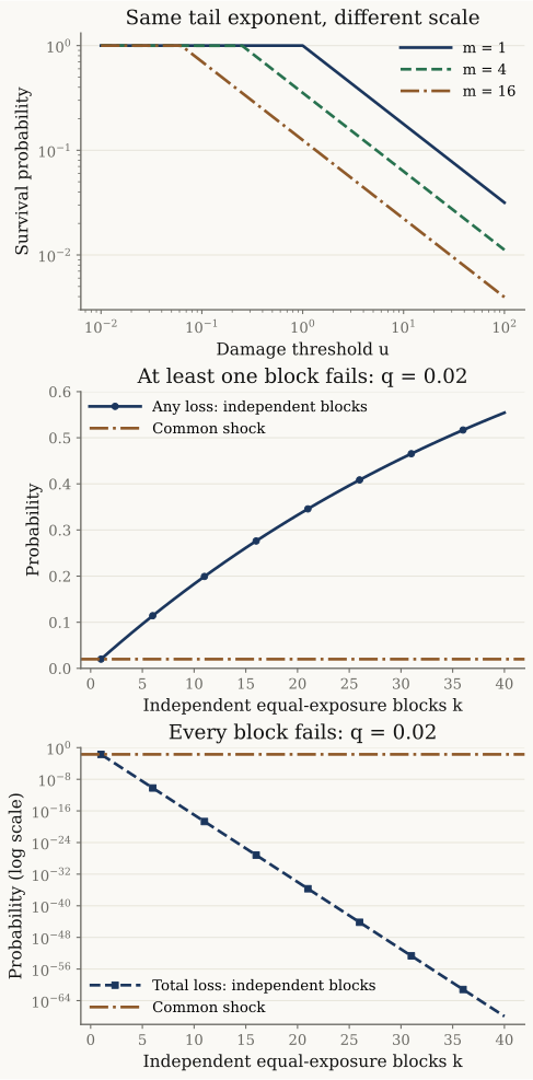
Top: exact survivals for , , and . Middle and bottom: bounded block failures at . A shared logarithmic axis would compress the any-loss and common-shock curves near its upper edge because total-loss probabilities reach about 10-68. Such apparent near-overlap is a scale effect: at , any loss has probability about 0.554, versus 0.02 under a common shock. They agree exactly at . Separate linear and logarithmic panels retain both comparisons. The Bernoulli model is bounded and is not heavy-tailed.
Use split_power_damage_logsf, block_failure_summary.
import numpy as np
from xmath.incerto.lecture_risk import split_power_damage_logsf, block_failure_summary

for modules in (1, 16):
    log_tail = split_power_damage_logsf(4, alpha=1.5, power=2, modules=modules)
    print(f"modules={modules:d}: {np.exp(log_tail):.4g}")
for blocks in (1, 10):
    print(f"blocks={blocks:d}")
    for name, value in block_failure_summary(0.02, blocks).items():
        print(f"  {name}: {value:.4g}")
Output
modules=1: 0.3536
modules=16: 0.04419
blocks=1
  mean: 0.02
  variance: 0.0196
  any_failure: 0.02
  total_failure: 0.02
blocks=10
  mean: 0.02
  variance: 0.00196
  any_failure: 0.1829
  total_failure: 1.024e-17
The split-damage calculation assumes equal modules; the block calculation assumes independent failures and equal exposures.
Figure regeneration: uv run python demos/incerto/lecture_risk.py. The script evaluates
161 thresholds from 0.01 to 100 and 40 block counts, prints the
worked cases, and generates the figure without sampling or external data.
The aggregation and response questions arise in Taleb (2025), ch. 3, §3.6.1, p. 53, and §3.12, pp. 66–67. The attached precaution paper, v1, §VII.A–C, p. 6, discusses nonlinear harm and dependence when splitting exposure. The convexity inequality, exact Pareto scaling and finite Bernoulli comparisons above are proved here under their stated models; they establish no general institutional or policy ranking.
- Taleb, N. N. (2025). Statistical Consequences of Fat Tails (3rd ed.). https://arxiv.org/abs/2001.10488v4