Reading a glossary through examples¶
A probability, a conditional mean, and a contribution to an expectation can all refer to observations above the same threshold. They answer different questions. This guide uses that distinction to connect the glossary to counting exceedances, the Pareto law, the extreme-value index, and the tail class catalog.
The source is Taleb (2025), Statistical Consequences of Fat Tails, third edition, arXiv:2001.10488v4, chapter 2, printed pp. 7–21. The tables give reading locations, not transcriptions of the glossary. Our examples and arguments are developed independently. The shared notation controls the symbols used here; source-specific conventions need translation.
Notation at the point of use¶
| Source term or symbol / locator | Our notation and meaning | Reading route |
|---|---|---|
| Probability, expectation, variance; §2.1, p. 7 | , , ; an expectation may be infinite or undefined | Pareto moment existence |
| Density; §2.1, p. 7 | for a parameterized density; local for a fixed Lebesgue density | Pareto definition |
| CDF and survival, , , ; §2.1, p. 7 | and | CDF and atoms |
| Sample size and sum; §2.1, pp. 7–8 | , , ; a hatted is instead a local empirical survival | Counting exceedances |
| Moment order ; §2.1, p. 7 | in for nonnegative ; use a separate local for a probability level | Moment thresholds |
| Tail and stable indices; §2.1, p. 8 | is the survival power exponent, the EVI; a stable-law index must be identified separately | Exact Pareto EVI proof |
| Threshold , lower endpoint ; §§2.2.1, 2.2.4, pp. 9–11 | is a threshold; is a Pareto minimum; | Conditional Pareto quantities |
| Gaussian scale and lognormal parameters; §2.1, p. 8 | Write with variance ; specify for a lognormal | Lognormal moments |
| Mean absolute deviation and normalized expression; §2.1, pp. 7–8 | State the center and normalization explicitly; $(n^{-1}\sum_i | x_i |
| Characteristic function, delta, step and special functions; §2.1, pp. 8–9 | Keep these local to the calculation; our remains a model parameter when used that way | Stable-limit characteristic functions; special-function identities need their own references |
For a lognormal, is a log-location, not its ordinary mean. The catalog derivation gives , so a prescribed mean requires . Likewise, the stable-law index is restricted to , whereas a Pareto exponent can exceed 2; neither is silently interchangeable with the EVI.
Map of the glossary concepts¶
The core route is probability → tail size → tail class → normalized extremes. Other glossary entries point ahead to later chapters. A link below identifies a relevant existing note, not a claim that all of that topic is proved here.
| Term / source locator | Our page or local interpretation |
|---|---|
| Power-law class; §2.2.1, p. 9 | Regular variation: has variation index |
| Weak LLN and CLT; §§2.2.2–3, p. 10 | The convergence statements below; preasymptotic averages distinguishes a limit from its finite-sample accuracy |
| Expected excess; §2.2.4, pp. 10–11 | Mean excess is ; conditional tail mean is |
| Medium numbers, preasymptotics; §§2.2.5, 2.2.17, pp. 11, 15 | Finite-sample averages; no universal convergence rate is supplied by naming the regime |
| Kappa; §2.2.6, pp. 11–12 | Planned chapter-8 treatment of dispersion scaling; a mean-centered formula needs an existing mean and finite, nonzero dispersion terms |
| Elliptical laws and independence; §§2.2.7–8, p. 12 | Mixtures supply examples; independence means a product joint law, and scatter need not be a finite covariance matrix |
| Stable and multivariate stable laws; §§2.2.9–10, pp. 12–13 | Generalized CLT; normalized sums and normalized maxima are different limit problems |
| Karamata point; §2.2.11, p. 13 | Counterexample to a constant tail factor; no finite transition point follows from slow variation |
| Subexponentiality; §2.2.12, pp. 13–14 | Subexponential tails; fix the number of iid nonnegative summands while the threshold tends to infinity |
| Student-t proxy; §2.2.13, p. 14 | Survival ratios; label degrees of freedom locally and distinguish this model from an exact Pareto |
| Stochasticizing, metaprobability; §§2.2.18, 2.2.31, pp. 15–16, 20 | Random-scale examples; a distribution over a parameter defines a mixture, with dependence specified separately |
| VaR and conditional VaR; §2.2.19, p. 16 | For a nonnegative loss , define a local quantile ; see the quantile and tail-mean distinction below |
| MS plot; §2.2.21, pp. 16–17 | Max-to-sum ratio; for moment order compare with , not with |
| Maximum domain of attraction; §2.2.22, p. 17 | EVI definition and Pareto proof; a nondegenerate normalized maximum limit is essential |
| Tail payoff integrals; §§2.2.23–24, pp. 17–18 | Tail contribution identity; omits the contribution above |
| Empirical distribution; §2.2.27, p. 19 | Strict counts; bounded indicator averages do not establish unbounded-moment convergence |
| Hidden tail and shadow moment; §§2.2.28–29, p. 20 | Plug-in estimation; the model assigns mass beyond the sample maximum, while a sample alone does not identify that mass |
| Tail dependence; §2.2.30, p. 20 | A limiting conditional exceedance probability at marginal quantiles, when the limit exists; dedicated multivariate treatment is planned |
| Dynamic hedging; §2.2.32, p. 21 | Planned Dynamic Hedging sequence; no replication theorem follows from the glossary alone |
| Citation ring, rent seeking, pseudo-empiricism, skin in the game, Wittgenstein’s ruler, Black Swans; §§2.2.14–16, 2.2.20, 2.2.25–26, pp. 14–19 | Interpretive source vocabulary, outside this chunk’s mathematical claims; no distributional theorem or empirical finding is inferred from these labels |
The normalized expression in the first table fails the triangle inequality when : for and it gives 1 for their sum but for the sum of their values. Independence can always be expressed by for measurable sets. A density ratio can express it only where the denominator is positive and the densities exist. An elliptical scatter matrix is a model parameter; identifying it with a covariance additionally requires second moments and the appropriate scalar normalization.
Which limit is being taken?¶
For random variables , convergence in probability means for every . Almost-sure convergence means . Convergence in distribution means convergence of the CDFs at continuity points of the limiting CDF. These are the conventions behind the arrows in §2.1, p. 8.
For iid with , the weak LLN gives , where . With the stronger assumption , the classical CLT gives
These two general theorems are cited, not proved here (SCoFT v4 §§2.2.2–3, p. 10). Neither statement gives a universal finite-sample error bound. The exceedance note does prove a pointwise probability bound for its bounded indicators.
By contrast, the subexponential relation compares and as with fixed. It does not say that tends to one as grows. The Pareto sums section keeps the growing-sample regimes and moment orders separate.
A probability does not specify the tail payoff¶
For Pareto , threshold is the quantile . The exceedance probability is , but the conditional mean above that threshold is 12. The Pareto derivation gives mean excess 8 and tail contribution . All four numbers describe the same distribution and threshold.
For an integrable nonnegative loss, define expected shortfall at level by . When there is no atom at the quantile, this agrees with the conditional tail mean. At an atom, conditioning on generally selects a different probability mass. For the empirical law of and , the upper half consists of equal masses at 2 and 4, so the quantile integral gives 3. Strict conditioning on instead gives 4. This calculation explains why the probability level, sign convention, and treatment of ties must accompany the terms VaR and expected shortfall.
Even uniform CDF accuracy does not control a mean without additional tail conditions. To prove this, let put mass at zero and at , for integers . Its CDF differs from that of a point mass at zero by at most , yet its mean is . This deterministic sequence of laws is a counterexample to such an implication; it is not a simulation of an iid empirical process. It isolates the probability-versus-moment issue behind §§2.2.27–28, pp. 19–20, without importing a uniform convergence theorem.
Reproduce the worked cases¶
Use empirical_survival_function, pareto_tail_quantities.
Code
from xmath.incerto.stats import empirical_survival_function
from xmath.incerto.glossary import pareto_tail_quantities

support, survival = empirical_survival_function([1, 2, 2, 4])
print("Support: [" + ", ".join(f"{v:.4g}" for v in support) + "]")
print("Strict survival: [" + ", ".join(f"{v:.4g}" for v in survival) + "]")
for alpha in (0.8, 1, 1.5, 3):
    result = pareto_tail_quantities(alpha, x_m=1, threshold=4)
    print(f"alpha={alpha:.4g}")
    for name, value in result.items():
        print(f"  {name}: {value:.4g}")
Output
Support: [1, 2, 4]
Strict survival: [0.75, 0.25, 0]
alpha=0.8
  log_survival: -1.109
  mean_excess: inf
  conditional_mean: inf
  tail_first_moment: inf
alpha=1
  log_survival: -1.386
  mean_excess: inf
  conditional_mean: inf
  tail_first_moment: inf
alpha=1.5
  log_survival: -2.079
  mean_excess: 8
  conditional_mean: 12
  tail_first_moment: 1.5
alpha=3
  log_survival: -4.159
  mean_excess: 2
  conditional_mean: 6
  tail_first_moment: 0.09375
Figure regeneration: uv run python demos/incerto/exceedances.py; uv run python demos/incerto/glossary_worked_cases.py.
The second script uses the fixed list and exact population formulas. It prints conditional Pareto quantities at for , the uniform-CDF counterexample for , and multiplier ratios for the catalog’s logarithmic correction. It evaluates four Pareto maximum CDFs with on 301 points from 0.25 to 4, and a 161-point multiplier grid from 1 to 104. Units are dimensionless. There is no RNG, external data, model fitting, or distribution truncation; the finite grids bound the work to a few seconds and two figure exports.
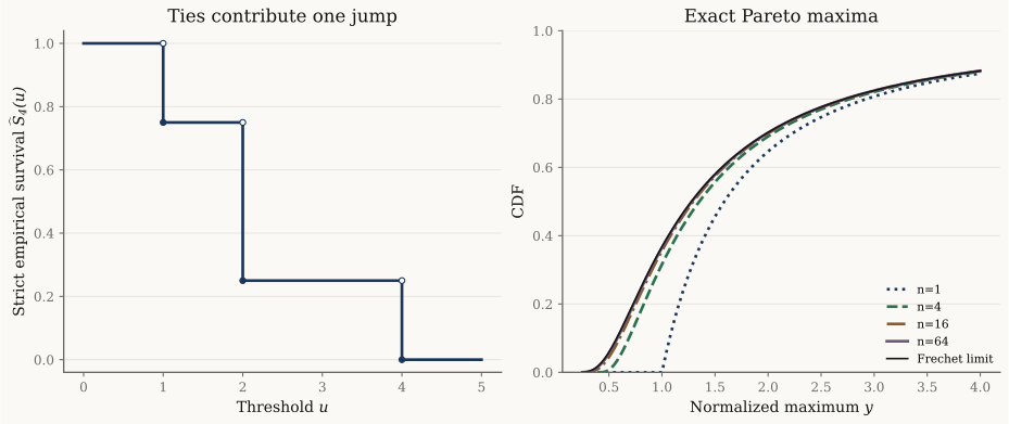
Left: the empirical law assigns half its mass to 2; closed circles mark the value after each downward jump. Right: exact iid Pareto maximum CDFs and their proved Fréchet limit. The finite curves illustrate the formulas; they are not estimates or evidence for an unknown population model.
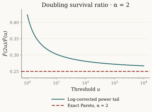
Both tails have exponent 2. The corrected law has , which grows without bound even as its multiplier ratio approaches the Pareto value. The catalog proves the limiting claim and validates the law.
Unexpected non-finite arithmetic raises an error. CDF values may round to zero or one at floating-point limits; this does not assert finite support. Tests compare finite formulas with independent integration and distribution calculations. The probability bounds, conditional identities, maximum limit, and counterexamples are proved in the notes, not by the tests.
References and next reading¶
Taleb, Statistical Consequences of Fat Tails, third edition (2025), arXiv:2001.10488v4, ch. 2, §§2.1–2.2.32, pp. 7–21. Section/page locators above identify source context.
Tail class catalog gives the precise classification sources and separates proved formulas from cited theorems.
Chapter 3 — Non-technical overview connects the definitions to statistical consequences; its source references retain the edition identified on that page.
- Taleb, N. N. (2025). Statistical Consequences of Fat Tails (3rd ed.). https://arxiv.org/abs/2001.10488v4