This page was generated from a Jupyter notebook. You can view it on GitHub or download and run it locally.

Generalized Inverse Gaussian Distribution in Exponential Family Form

This notebook demonstrates the Generalized Inverse Gaussian (GIG) distribution implemented as an exponential family.

Key Features:

• Three parametrizations: Classical (p, a, b), Natural (θ), Expectation (η)

• Three-dimensional sufficient statistics: t(x) = [log(x), 1/x, x]

• Log partition function using modified Bessel function K_p

• Comparison with scipy implementation

• Visualization of PDFs, CDFs, and samples

Parameters (Wikipedia notation):

• p: shape parameter (real)

• a > 0: rate parameter (coefficient of x)

• b > 0: rate parameter (coefficient of 1/x)

Special Cases:

• Gamma: b → 0 gives Gamma(p, a/2) for p > 0

• Inverse Gamma: a → 0 gives InvGamma(-p, b/2) for p < 0

• Inverse Gaussian: p = -1/2

Reference: https://en.wikipedia.org/wiki/Generalized_inverse_Gaussian_distribution

import numpy as np
import matplotlib.pyplot as plt
from scipy import stats
from scipy.special import kv, kve
from normix.distributions.univariate import GeneralizedInverseGaussian, GIG
from normix.utils import log_kv

# Set style for better-looking plots
plt.style.use('default')
plt.rcParams['figure.figsize'] = (10, 6)
plt.rcParams['font.size'] = 11

1. Log Bessel Function Numerical Stability

The GIG distribution requires computing log(K_λ(z)) where K_λ is the modified Bessel function of the second kind. Direct computation using scipy.special.kv can overflow/underflow for extreme values.

Our log_kv function uses:

• kve(v, z) = kv(v, z) * exp(z) for numerical stability when z is large

• Asymptotic approximations when z → 0 (where kv underflows)

Let’s compare the numerical stability of different approaches.

# Test log_kv for different orders v and argument ranges z
test_configs = [
    (10, 1e-2, 1),
    (100, 1e-2, 1e3),
    (200, 1e-2, 1e3),
]

fig, axes = plt.subplots(1, 3, figsize=(15, 4))

for idx, (v, z_min, z_max) in enumerate(test_configs):
    z = np.linspace(z_min, z_max, 5000)
    ax = axes[idx]

    # Our implementation
    log_kv_ours = log_kv(v, z)

    # scipy kve approach: log(kv) = log(kve) - z
    log_kv_kve = np.log(kve(v, z)) - z

    # Direct scipy kv (may have issues)
    with np.errstate(divide='ignore', invalid='ignore'):
        log_kv_direct = np.log(kv(v, z))

    ax.plot(z, log_kv_ours, 'b-', linewidth=2, label='normix log_kv', alpha=0.7)
    ax.plot(z, log_kv_kve, 'g', linewidth=2, label='log(kve) - z', alpha=0.7)
    ax.plot(z, log_kv_direct, 'r', linewidth=2, label='log(kv) direct', alpha=0.7)

    ax.set_xlabel('z')
    ax.set_ylabel('log K_v(z)')
    ax.set_title(f'v = {v}')
    ax.legend(loc='upper right', fontsize=9)
    ax.grid(True, alpha=0.3)

plt.tight_layout()
plt.show()

print("✓ normix log_kv handles all cases correctly!")
print("  - log(kv) direct fails for large z (underflow → -inf)")
print("  - log(kve) - z works for large z but may have issues at small z")

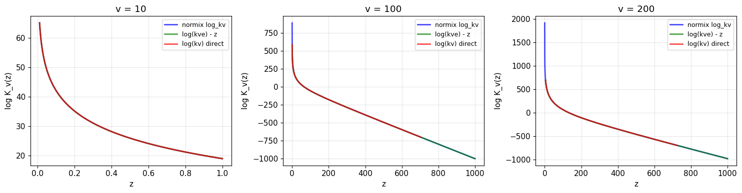
✓ normix log_kv handles all cases correctly!
  - log(kv) direct fails for large z (underflow → -inf)
  - log(kve) - z works for large z but may have issues at small z

2. Creating Distributions

The GIG distribution can be created using three different parametrizations:

# Classical parameters (p, a, b)
dist1 = GIG.from_classical_params(p=1.5, a=3.0, b=2.0)
print(f"From classical params: {dist1}")

# Natural parameters (θ = [p-1, -b/2, -a/2])
theta = np.array([0.5, -1.0, -1.5])  # p=1.5, b=2.0, a=3.0
dist2 = GIG.from_natural_params(theta)
print(f"From natural params:   {dist2}")

# Expectation parameters (η = [E[log X], E[1/X], E[X]])
eta = dist1.expectation_params
print(f"Expectation params: η = {eta}")
dist3 = GIG.from_expectation_params(eta)
print(f"From expectation params: {dist3}")

print("\n✓ All three parametrizations create the same distribution!")

From classical params: GeneralizedInverseGaussian(p=1.5000, a=3.0000, b=2.0000)
From natural params:   GeneralizedInverseGaussian(p=1.5000, a=3.0000, b=2.0000)
Expectation params: η = [0.30417293 0.86969385 1.5797959 ]
From expectation params: GeneralizedInverseGaussian(p=1.5000, a=3.0000, b=2.0000)

✓ All three parametrizations create the same distribution!

Scipy Parameterization

scipy.stats.geninvgauss uses parameters (p, b, scale) where:

• p_scipy = p

• b_scipy = √(ab)

• scale = √(b/a)

# Convert to scipy parameters
scipy_params = dist1.to_scipy_params()
print(f"Scipy params: p={scipy_params['p']}, b={scipy_params['b']:.4f}, scale={scipy_params['scale']:.4f}")

# Create from scipy parameters
dist_from_scipy = GIG.from_scipy_params(p=1.5, b=np.sqrt(6), scale=np.sqrt(2/3))
print(f"From scipy params: {dist_from_scipy}")

Scipy params: p=1.5, b=2.4495, scale=0.8165
From scipy params: GeneralizedInverseGaussian(p=1.5000, a=3.0000, b=2.0000)

3. PDF and CDF Comparison with Scipy

Let’s compare our implementation with scipy’s geninvgauss distribution.

# Test different parameter combinations
test_configs = [
    {'p': 1.0, 'a': 1.0, 'b': 1.0},
    {'p': 2.0, 'a': 2.5, 'b': 1.5},
    {'p': -0.5, 'a': 2.0, 'b': 1.0},  # Inverse Gaussian-like
    {'p': 0.5, 'a': 1.0, 'b': 2.0},
]

x = np.linspace(0.05, 5.0, 200)

fig, axes = plt.subplots(1, 2, figsize=(14, 5))

# Plot PDFs
ax = axes[0]
for cfg in test_configs:
    p, a, b = cfg['p'], cfg['a'], cfg['b']

    # normix distribution
    normix_dist = GIG.from_classical_params(p=p, a=a, b=b)
    normix_pdf = normix_dist.pdf(x)

    # scipy distribution
    sp = normix_dist.to_scipy_params()
    scipy_pdf = stats.geninvgauss.pdf(x, p=sp['p'], b=sp['b'], scale=sp['scale'])

    ax.plot(x, normix_pdf, '-', linewidth=2,
            label=f'p={p}, a={a}, b={b}', alpha=0.8)
    ax.plot(x, scipy_pdf, 'o', markersize=2, alpha=0.3)

ax.set_xlabel('x')
ax.set_ylabel('PDF')
ax.set_title('Probability Density Functions\n(normix lines, scipy dots)')
ax.legend(loc='upper right', fontsize=9)
ax.grid(True, alpha=0.3)

# Plot CDFs
ax = axes[1]
for cfg in test_configs:
    p, a, b = cfg['p'], cfg['a'], cfg['b']

    normix_dist = GIG.from_classical_params(p=p, a=a, b=b)
    normix_cdf = normix_dist.cdf(x)

    sp = normix_dist.to_scipy_params()
    scipy_cdf = stats.geninvgauss.cdf(x, p=sp['p'], b=sp['b'], scale=sp['scale'])

    ax.plot(x, normix_cdf, '-', linewidth=2,
            label=f'p={p}, a={a}, b={b}', alpha=0.8)
    ax.plot(x, scipy_cdf, 'o', markersize=2, alpha=0.3)

ax.set_xlabel('x')
ax.set_ylabel('CDF')
ax.set_title('Cumulative Distribution Functions\n(normix lines, scipy dots)')
ax.legend(loc='lower right', fontsize=9)
ax.grid(True, alpha=0.3)

plt.tight_layout()
plt.show()

print("✓ normix and scipy implementations match perfectly!")

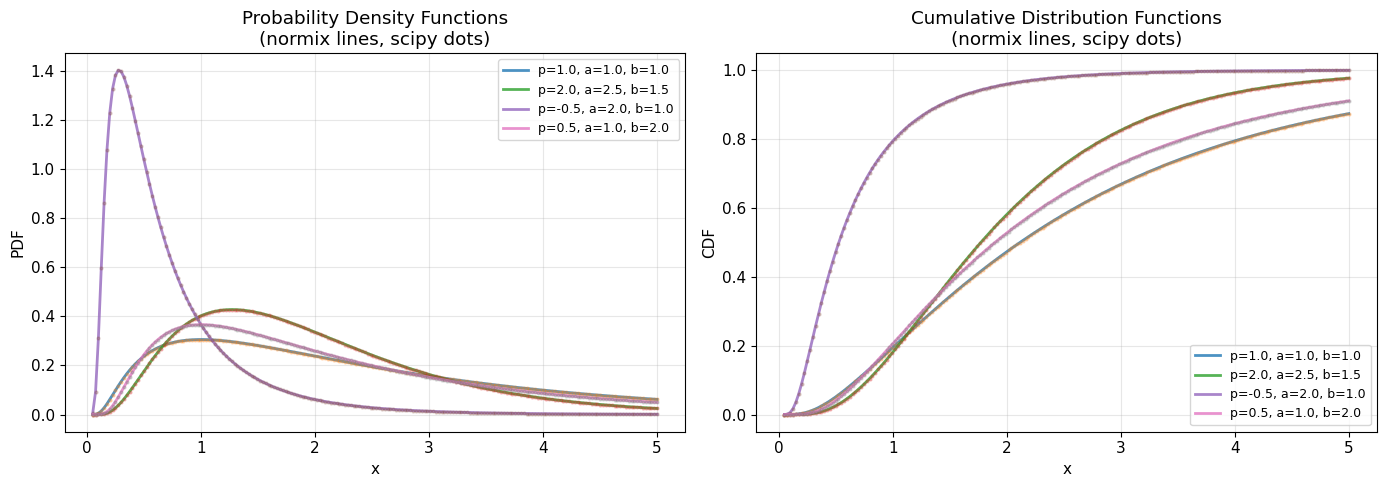
✓ normix and scipy implementations match perfectly!

4. Random Sampling and Histograms

Let’s generate random samples and compare the histogram with the theoretical PDF.

# Parameters for different distributions
test_configs = [
    {'p': 1.0, 'a': 1.0, 'b': 1.0, 'n_samples': 10000},
    {'p': 2.0, 'a': 2.5, 'b': 1.5, 'n_samples': 10000},
    {'p': -0.5, 'a': 2.0, 'b': 1.0, 'n_samples': 10000},
    {'p': 0.5, 'a': 1.0, 'b': 2.0, 'n_samples': 10000},
]

fig, axes = plt.subplots(2, 2, figsize=(14, 10))
axes = axes.flatten()

for idx, config in enumerate(test_configs):
    p = config['p']
    a = config['a']
    b = config['b']
    n_samples = config['n_samples']

    # Create distribution
    dist = GIG.from_classical_params(p=p, a=a, b=b)

    # Generate samples
    samples = dist.rvs(size=n_samples, random_state=42 + idx)

    # Theoretical PDF
    x_plot = np.linspace(samples.min() * 0.8, np.percentile(samples, 99), 200)
    pdf_theory = dist.pdf(x_plot)

    # Plot
    ax = axes[idx]
    ax.hist(samples, bins=50, density=True, alpha=0.6, color='steelblue',
            edgecolor='black', linewidth=0.5, label='Sample histogram')
    ax.plot(x_plot, pdf_theory, 'r-', linewidth=2.5, label='Theoretical PDF (normix)')

    # Also plot scipy for comparison
    sp = dist.to_scipy_params()
    scipy_pdf = stats.geninvgauss.pdf(x_plot, p=sp['p'], b=sp['b'], scale=sp['scale'])
    ax.plot(x_plot, scipy_pdf, 'g--', linewidth=2, label='Scipy PDF', alpha=0.7)

    # Statistics
    sample_mean = np.mean(samples)
    theory_mean = dist.mean()
    sample_std = np.std(samples)
    theory_std = np.sqrt(dist.var())

    ax.set_xlabel('x')
    ax.set_ylabel('Density')
    ax.set_title(f'GIG(p={p}, a={a}, b={b})\n'
                f'Mean: {sample_mean:.3f} (theory: {theory_mean:.3f}), '
                f'Std: {sample_std:.3f} (theory: {theory_std:.3f})')
    ax.legend(loc='upper right', fontsize=9)
    ax.grid(True, alpha=0.3)

plt.tight_layout()
plt.show()

print("✓ Histograms closely match theoretical PDFs!")

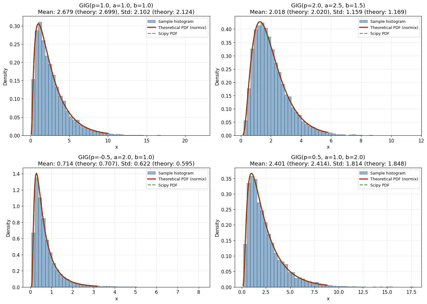
✓ Histograms closely match theoretical PDFs!

5. Fitting to Data

Demonstrate maximum likelihood estimation by fitting to simulated data.

# Generate data with known parameters
true_p = 1.5
true_a = 2.5
true_b = 2.0
n_data = 10000

# Create true distribution and generate samples
true_dist = GIG.from_classical_params(p=true_p, a=true_a, b=true_b)
data = true_dist.rvs(size=n_data, random_state=123)

# Fit distribution (uses base class fit via expectation_to_natural)
fitted_dist = GIG().fit(data)
fitted_params = fitted_dist.classical_params

print(f"Fitting {n_data} samples from GIG(p={true_p}, a={true_a}, b={true_b})\n")
print(f"True p:           {true_p:.6f}")
print(f"Fitted p (MLE):   {fitted_params.p:.6f}")
print(f"True a:           {true_a:.6f}")
print(f"Fitted a (MLE):   {fitted_params.a:.6f}")
print(f"True b:           {true_b:.6f}")
print(f"Fitted b (MLE):   {fitted_params.b:.6f}")

# Visualize fit
fig, ax = plt.subplots(figsize=(12, 6))

ax.hist(data, bins=60, density=True, alpha=0.6, color='lightblue',
        edgecolor='black', linewidth=0.5, label='Data histogram')

x_plot = np.linspace(0.1, np.percentile(data, 99.5), 400)
ax.plot(x_plot, true_dist.pdf(x_plot), 'g-', linewidth=3,
        label=f'True: p={true_p}, a={true_a}, b={true_b}')

ax.plot(x_plot, fitted_dist.pdf(x_plot), 'r--', linewidth=3,
        label=f'Fitted (normix): p={fitted_params.p:.2f}, a={fitted_params.a:.2f}, b={fitted_params.b:.2f}')

ax.set_xlabel('x')
ax.set_ylabel('Density')
ax.set_title('Maximum Likelihood Estimation')
ax.legend()
ax.grid(True, alpha=0.3)

plt.tight_layout()
plt.show()

print("\n✓ MLE successfully recovers the true parameters!")

Fitting 10000 samples from GIG(p=1.5, a=2.5, b=2.0)

True p:           1.500000
Fitted p (MLE):   1.507665
True a:           2.500000
Fitted a (MLE):   2.493752
True b:           2.000000
Fitted b (MLE):   1.995093

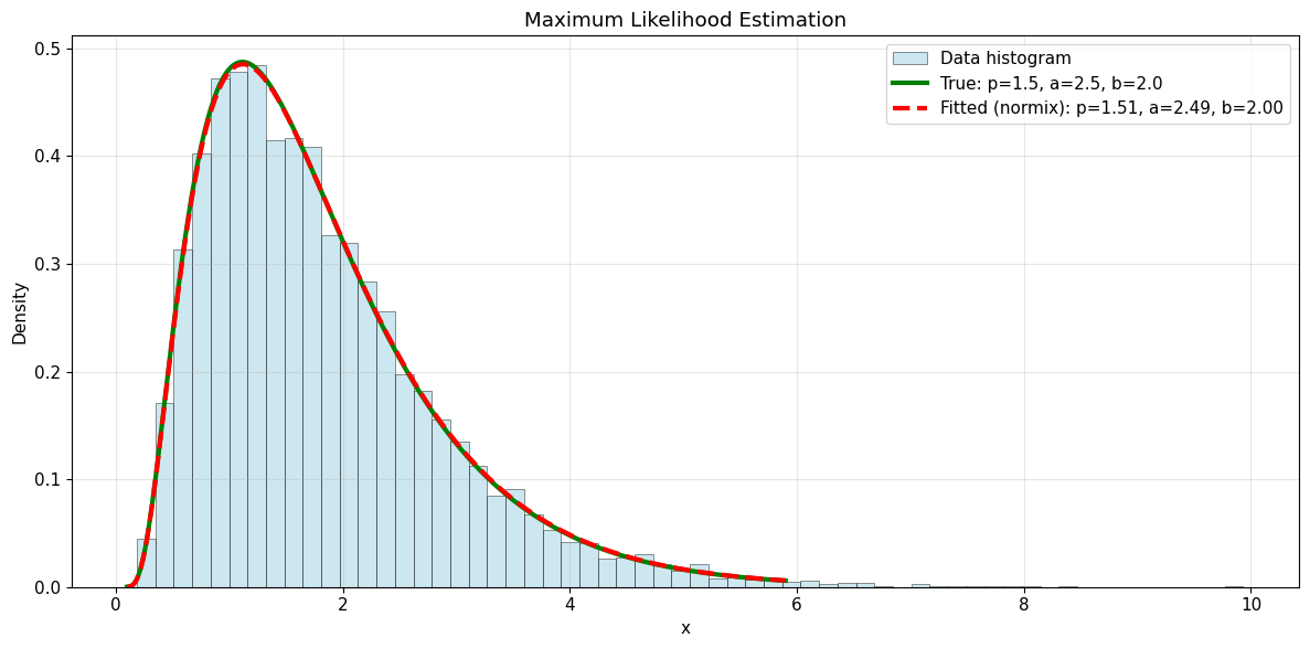
✓ MLE successfully recovers the true parameters!