This page was generated from a Jupyter notebook. You can view it on GitHub or download and run it locally.

Multivariate Normal Distribution in Exponential Family Form

This notebook demonstrates the Multivariate Normal distribution implemented as an exponential family.

Key Features:

• Three parametrizations: Classical (μ, Σ), Natural (θ), Expectation (η)

• Sufficient statistics: t(x) = [x, xx^T]

• Supports both univariate (d=1) and multivariate (d>1) cases

• Comparison with scipy implementation

• Visualization of PDFs, CDFs, and samples

import numpy as np
import matplotlib.pyplot as plt
from scipy import stats
from normix.distributions.multivariate import MultivariateNormal

# Set style for better-looking plots
plt.style.use('default')
plt.rcParams['figure.figsize'] = (10, 6)
plt.rcParams['font.size'] = 11

1. Creating Distributions (1D Case)

The multivariate normal distribution can be created using three different parametrizations. Let’s first look at the 1D (univariate) case:

# Classical parameters (μ, Σ)
mu = np.array([2.0])
sigma = np.array([[1.5]])

dist1 = MultivariateNormal.from_classical_params(mu=mu, sigma=sigma)
print(f"From classical params: {dist1}")

# Natural parameters
theta = dist1.natural_params
dist2 = MultivariateNormal(d=1).from_natural_params(theta)
print(f"From natural params:   {dist2}")

# Expectation parameters
eta = dist1.expectation_params
dist3 = MultivariateNormal(d=1).from_expectation_params(eta)
print(f"From expectation params: {dist3}")

print("\n✓ All three parametrizations create the same distribution!")

From classical params: MultivariateNormal(μ=2.0000, σ²=1.5000)
From natural params:   MultivariateNormal(μ=2.0000, σ²=1.5000)
From expectation params: MultivariateNormal(μ=2.0000, σ²=1.5000)

✓ All three parametrizations create the same distribution!

2. PDF and CDF Comparison with Scipy (1D Case)

Let’s compare our implementation with scipy’s normal distribution.

# Test different parameter combinations
test_configs = [
    {'mu': np.array([0.0]), 'sigma': np.array([[1.0]])},
    {'mu': np.array([2.0]), 'sigma': np.array([[0.5]])},
    {'mu': np.array([-1.0]), 'sigma': np.array([[2.0]])},
    {'mu': np.array([1.0]), 'sigma': np.array([[0.25]])},
]

x = np.linspace(-5, 5, 200)

fig, axes = plt.subplots(1, 2, figsize=(14, 5))

# Plot PDFs
ax = axes[0]
for cfg in test_configs:
    mu_val = cfg['mu'][0]
    sigma_val = cfg['sigma'][0, 0]

    # normix distribution
    normix_dist = MultivariateNormal.from_classical_params(**cfg)
    normix_pdf = normix_dist.pdf(x.reshape(-1, 1))

    # scipy distribution
    scipy_dist = stats.norm(loc=mu_val, scale=np.sqrt(sigma_val))
    scipy_pdf = scipy_dist.pdf(x)

    # Plot both
    ax.plot(x, normix_pdf, '-', linewidth=2,
            label=f'μ={mu_val:.1f}, σ²={sigma_val:.2f}', alpha=0.8)
    ax.plot(x, scipy_pdf, 'o', markersize=2, alpha=0.3)

ax.set_xlabel('x')
ax.set_ylabel('PDF')
ax.set_title('Probability Density Functions\n(normix lines, scipy dots)')
ax.legend(loc='upper right', fontsize=9)
ax.grid(True, alpha=0.3)

# Plot CDFs
ax = axes[1]
for cfg in test_configs:
    mu_val = cfg['mu'][0]
    sigma_val = cfg['sigma'][0, 0]

    # normix distribution
    normix_dist = MultivariateNormal.from_classical_params(**cfg)
    normix_cdf = normix_dist.cdf(x)

    # scipy distribution
    scipy_dist = stats.norm(loc=mu_val, scale=np.sqrt(sigma_val))
    scipy_cdf = scipy_dist.cdf(x)

    # Plot both
    ax.plot(x, normix_cdf, '-', linewidth=2,
            label=f'μ={mu_val:.1f}, σ²={sigma_val:.2f}', alpha=0.8)
    ax.plot(x, scipy_cdf, 'o', markersize=2, alpha=0.3)

ax.set_xlabel('x')
ax.set_ylabel('CDF')
ax.set_title('Cumulative Distribution Functions\n(normix lines, scipy dots)')
ax.legend(loc='lower right', fontsize=9)
ax.grid(True, alpha=0.3)

plt.tight_layout()
plt.show()

print("✓ normix and scipy implementations match perfectly!")

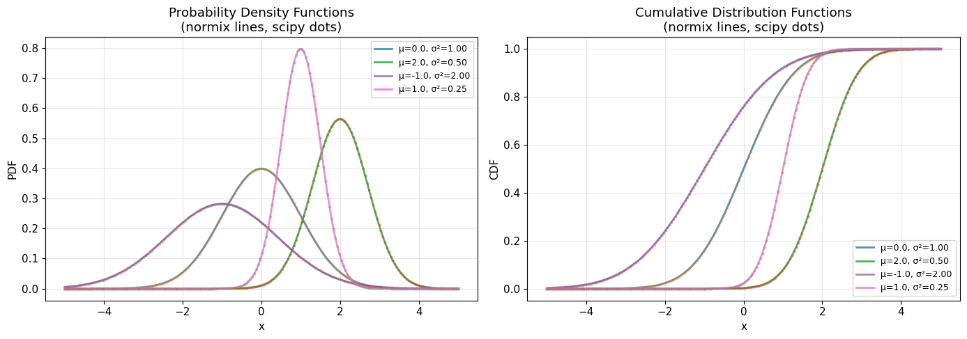
✓ normix and scipy implementations match perfectly!

3. Random Sampling and Histograms (1D Case)

Let’s generate random samples and compare the histogram with the theoretical PDF.

# Parameters for different distributions
test_configs = [
    {'mu': np.array([0.0]), 'sigma': np.array([[1.0]]), 'n_samples': 10000},
    {'mu': np.array([2.0]), 'sigma': np.array([[0.5]]), 'n_samples': 10000},
    {'mu': np.array([-1.0]), 'sigma': np.array([[2.0]]), 'n_samples': 10000},
    {'mu': np.array([1.0]), 'sigma': np.array([[0.25]]), 'n_samples': 10000},
]

fig, axes = plt.subplots(2, 2, figsize=(14, 10))
axes = axes.flatten()

for idx, config in enumerate(test_configs):
    mu = config['mu']
    sigma = config['sigma']
    n_samples = config['n_samples']

    dist = MultivariateNormal.from_classical_params(mu=mu, sigma=sigma)
    samples = dist.rvs(size=n_samples, random_state=42 + idx)
    samples_flat = samples.flatten()

    x_plot = np.linspace(samples_flat.min() - 0.5, samples_flat.max() + 0.5, 200)
    pdf_theory = dist.pdf(x_plot.reshape(-1, 1))

    ax = axes[idx]
    ax.hist(samples_flat, bins=50, density=True, alpha=0.6, color='steelblue',
            edgecolor='black', linewidth=0.5, label='Sample histogram')
    ax.plot(x_plot, pdf_theory, 'r-', linewidth=2.5, label='Theoretical PDF (normix)')

    scipy_dist = stats.norm(loc=mu[0], scale=np.sqrt(sigma[0, 0]))
    ax.plot(x_plot, scipy_dist.pdf(x_plot), 'g--', linewidth=2, label='Scipy PDF', alpha=0.7)

    sample_mean = np.mean(samples_flat)
    theory_mean = dist.mean()[0]
    sample_std = np.std(samples_flat)
    theory_std = np.sqrt(dist.var()[0])

    ax.set_xlabel('x')
    ax.set_ylabel('Density')
    ax.set_title(f'Normal(μ={mu[0]:.1f}, σ²={sigma[0,0]:.2f})\n'
                f'Mean: {sample_mean:.3f} (theory: {theory_mean:.3f}), '
                f'Std: {sample_std:.3f} (theory: {theory_std:.3f})')
    ax.legend(loc='upper right', fontsize=9)
    ax.grid(True, alpha=0.3)

plt.tight_layout()
plt.show()
print("✓ Histograms match theoretical PDFs closely!")

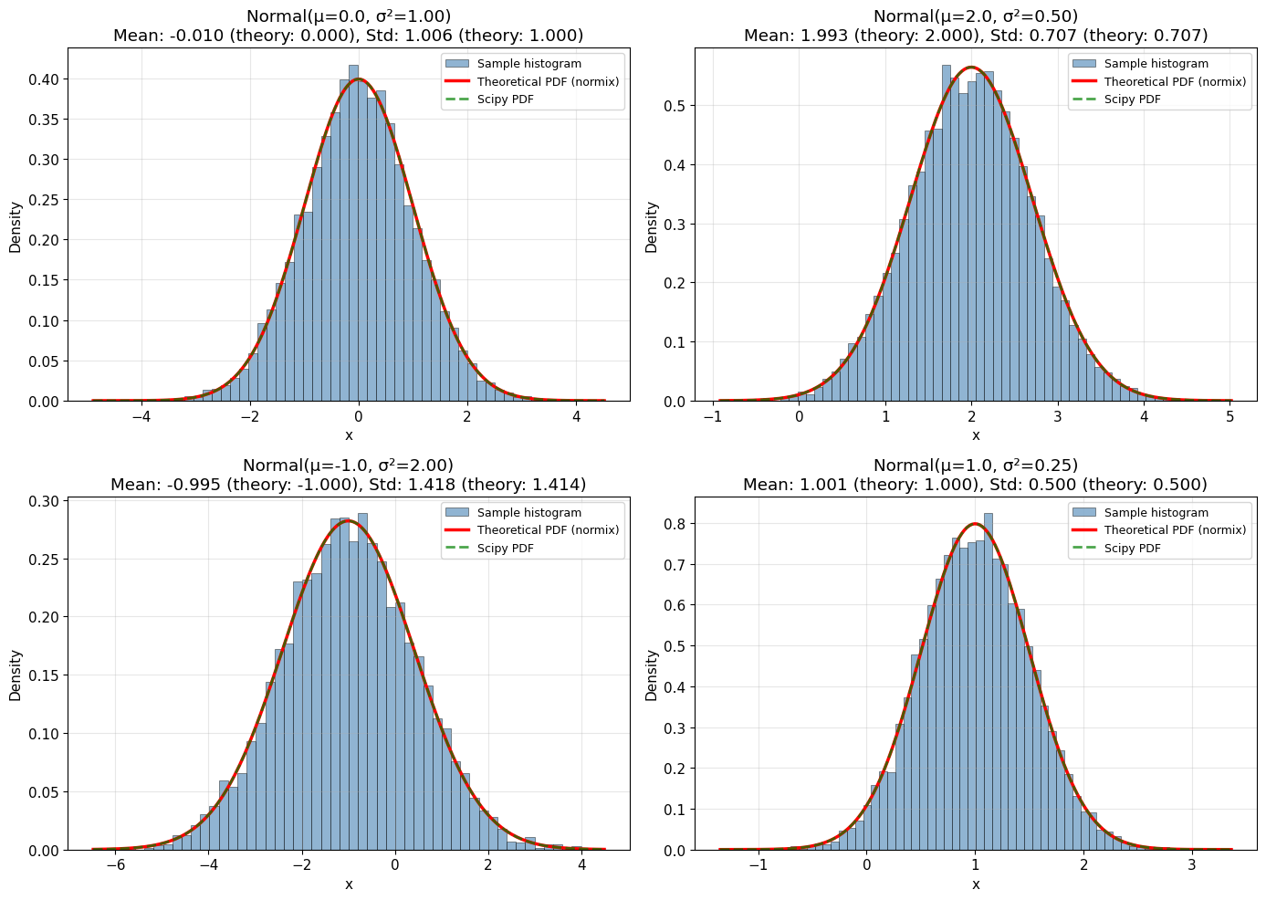
✓ Histograms match theoretical PDFs closely!

4. Two-Dimensional Case: Scatter Plot vs PDF Contour

Now let’s visualize the 2D multivariate normal distribution.

# Create 2D distribution with correlation
mu_2d = np.array([1.0, 2.0])
sigma_2d = np.array([[1.0, 0.6],
                     [0.6, 1.5]])

dist_2d = MultivariateNormal.from_classical_params(mu=mu_2d, sigma=sigma_2d)
print(f"2D Distribution: {dist_2d}")
print(f"Mean: {dist_2d.mean()}")
print(f"Covariance:\n{dist_2d.cov()}")

2D Distribution: MultivariateNormal(μ=[1.0000, 2.0000], d=2)
Mean: [1. 2.]
Covariance:
[[1.  0.6]
 [0.6 1.5]]

# Generate samples
n_samples = 2000
samples_2d = dist_2d.rvs(size=n_samples, random_state=42)

# Create grid for PDF contour
x1_range = np.linspace(mu_2d[0] - 3*np.sqrt(sigma_2d[0,0]),
                       mu_2d[0] + 3*np.sqrt(sigma_2d[0,0]), 100)
x2_range = np.linspace(mu_2d[1] - 3*np.sqrt(sigma_2d[1,1]),
                       mu_2d[1] + 3*np.sqrt(sigma_2d[1,1]), 100)
X1, X2 = np.meshgrid(x1_range, x2_range)
grid_points = np.column_stack([X1.ravel(), X2.ravel()])

# Compute PDF on grid
pdf_values = dist_2d.pdf(grid_points).reshape(X1.shape)
scipy_2d = stats.multivariate_normal(mean=mu_2d, cov=sigma_2d)
scipy_pdf = scipy_2d.pdf(grid_points).reshape(X1.shape)

fig, axes = plt.subplots(1, 3, figsize=(18, 6))

# Scatter plot with contours
ax = axes[0]
ax.scatter(samples_2d[:, 0], samples_2d[:, 1], alpha=0.3, s=10, c='steelblue', label='Samples')
contour = ax.contour(X1, X2, pdf_values, levels=8, colors='red', linewidths=1.5)
ax.clabel(contour, inline=True, fontsize=8, fmt='%.3f')
ax.scatter([mu_2d[0]], [mu_2d[1]], color='red', marker='x', s=200, linewidths=3, label='Mean')
ax.set_xlabel('x₁')
ax.set_ylabel('x₂')
ax.set_title(f'Scatter Plot with PDF Contours\n(n={n_samples} samples, normix)')
ax.legend()
ax.grid(True, alpha=0.3)
ax.set_aspect('equal')

# PDF heatmap
ax = axes[1]
im = ax.pcolormesh(X1, X2, pdf_values, shading='auto', cmap='viridis')
ax.contour(X1, X2, pdf_values, levels=8, colors='white', linewidths=0.5, alpha=0.7)
ax.scatter([mu_2d[0]], [mu_2d[1]], color='red', marker='x', s=200, linewidths=3)
plt.colorbar(im, ax=ax, label='PDF')
ax.set_xlabel('x₁')
ax.set_ylabel('x₂')
ax.set_title('PDF Heatmap (normix)')
ax.set_aspect('equal')

# PDF comparison
ax = axes[2]
ax.contour(X1, X2, pdf_values, levels=8, colors='blue', linewidths=2, linestyles='-')
ax.contour(X1, X2, scipy_pdf, levels=8, colors='red', linewidths=1, linestyles='--')
ax.scatter([mu_2d[0]], [mu_2d[1]], color='green', marker='x', s=200, linewidths=3)
ax.set_xlabel('x₁')
ax.set_ylabel('x₂')
ax.set_title('PDF Comparison\n(normix solid blue, scipy dashed red)')
ax.grid(True, alpha=0.3)
ax.set_aspect('equal')

plt.tight_layout()
plt.show()

max_diff = np.max(np.abs(pdf_values - scipy_pdf))
print(f"\n✓ Maximum PDF difference between normix and scipy: {max_diff:.2e}")
print("✓ The contours overlap perfectly!")

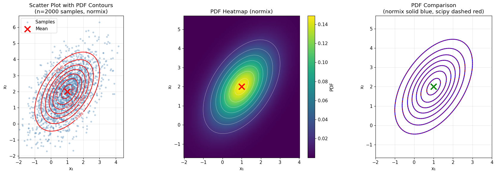
✓ Maximum PDF difference between normix and scipy: 8.33e-17
✓ The contours overlap perfectly!

5. Fitting to Data

Demonstrate maximum likelihood estimation by fitting to 2D data.

# Generate data with known parameters
true_mu = np.array([1.5, -0.5])
true_sigma = np.array([[2.0, 0.8], [0.8, 1.5]])
n_data = 2000

true_dist = MultivariateNormal.from_classical_params(mu=true_mu, sigma=true_sigma)
data = true_dist.rvs(size=n_data, random_state=123)

# Fit distribution
fitted_dist = MultivariateNormal(d=2).fit(data)
fitted_params = fitted_dist.classical_params

print(f"Fitting {n_data} samples\n")
print("True mean:", true_mu)
print("Fitted mean:", fitted_params.mu)
print("\nTrue covariance:\n", true_sigma)
print("Fitted covariance:\n", fitted_params.sigma)

# Visualize
x1_range = np.linspace(-3, 6, 100)
x2_range = np.linspace(-4, 3, 100)
X1, X2 = np.meshgrid(x1_range, x2_range)
grid = np.column_stack([X1.ravel(), X2.ravel()])

true_pdf = true_dist.pdf(grid).reshape(X1.shape)
fitted_pdf = fitted_dist.pdf(grid).reshape(X1.shape)

fig, ax = plt.subplots(figsize=(10, 8))
ax.scatter(data[:, 0], data[:, 1], alpha=0.2, s=5, c='lightgray', label='Data')
ax.contour(X1, X2, true_pdf, levels=6, colors='green', linewidths=2, linestyles='--', label='True')
ax.contour(X1, X2, fitted_pdf, levels=6, colors='red', linewidths=2, label='Fitted')
ax.scatter([true_mu[0]], [true_mu[1]], color='green', marker='x', s=200, linewidths=3)
ax.scatter([fitted_params.mu[0]], [fitted_params.mu[1]], color='red', marker='+', s=200, linewidths=3)
ax.set_xlabel('x₁')
ax.set_ylabel('x₂')
ax.set_title('Fitted vs True Distribution\n(green dashed: true, red solid: fitted)')
ax.grid(True, alpha=0.3)
ax.set_aspect('equal')
plt.tight_layout()
plt.show()

print("\n✓ MLE successfully recovers the true parameters!")

Fitting 2000 samples

True mean: [ 1.5 -0.5]
Fitted mean: [ 1.52481139 -0.49959382]

True covariance:
 [[2.  0.8]
 [0.8 1.5]]
Fitted covariance:
 [[2.01448169 0.83246155]
 [0.83246155 1.55148127]]

/tmp/ipykernel_2337733/1821489505.py:30: UserWarning: The following kwargs were not used by contour: 'label'
  ax.contour(X1, X2, true_pdf, levels=6, colors='green', linewidths=2, linestyles='--', label='True')
/tmp/ipykernel_2337733/1821489505.py:31: UserWarning: The following kwargs were not used by contour: 'label'
  ax.contour(X1, X2, fitted_pdf, levels=6, colors='red', linewidths=2, label='Fitted')

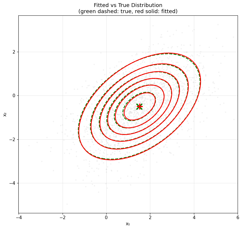
✓ MLE successfully recovers the true parameters!