This page was generated from a Jupyter notebook. You can view it on GitHub or download and run it locally.

Inverse Gamma Distribution in Exponential Family Form

This notebook demonstrates the Inverse Gamma distribution implemented as an exponential family.

Key Features:

• Three parametrizations: Classical (shape α, rate β), Natural (θ), Expectation (η)

• Two-dimensional sufficient statistics: t(x) = [-1/x, log(x)]

• Analytical formulas for gradients and Fisher information

• Comparison with scipy implementation

• Visualization of PDFs, CDFs, and samples

import numpy as np
import matplotlib.pyplot as plt
from scipy import stats
from normix.distributions.univariate import InverseGamma

# Set style for better-looking plots
plt.style.use('default')
plt.rcParams['figure.figsize'] = (10, 6)
plt.rcParams['font.size'] = 11

1. Creating Distributions

The inverse gamma distribution can be created using three different parametrizations:

# Classical parameters (shape α, rate β)
dist1 = InverseGamma.from_classical_params(shape=3.0, rate=1.5)
print(f"From classical params: {dist1}")

# Natural parameters (θ = [β, -(α+1)])
dist2 = InverseGamma.from_natural_params(np.array([1.5, -4.0]))
print(f"From natural params:   {dist2}")

# Expectation parameters
eta = dist1.expectation_params
dist3 = InverseGamma.from_expectation_params(eta)
print(f"From expectation params: {dist3}")

print("\n✓ All three parametrizations create the same distribution!")

From classical params: InverseGamma(shape=3.0000, rate=1.5000)
From natural params:   InverseGamma(shape=3.0000, rate=1.5000)
From expectation params: InverseGamma(shape=3.0000, rate=1.5000)

✓ All three parametrizations create the same distribution!

2. PDF and CDF Comparison with Scipy

Let’s compare our implementation with scipy’s inverse gamma distribution.

# Test different parameter combinations
test_configs = [
    {'shape': 3.0, 'rate': 1.0},
    {'shape': 3.0, 'rate': 2.0},
    {'shape': 5.0, 'rate': 1.0},
    {'shape': 5.0, 'rate': 2.0}
]

x = np.linspace(0.01, 5, 200)

fig, axes = plt.subplots(1, 2, figsize=(14, 5))

# Plot PDFs
ax = axes[0]
for cfg in test_configs:
    shape, rate = cfg['shape'], cfg['rate']

    # normix distribution
    normix_dist = InverseGamma.from_classical_params(shape=shape, rate=rate)
    normix_pdf = normix_dist.pdf(x)

    # scipy distribution
    scipy_dist = stats.invgamma(a=shape, scale=rate)
    scipy_pdf = scipy_dist.pdf(x)

    # Plot both (lines should overlap)
    ax.plot(x, normix_pdf, '-', linewidth=2,
            label=f'α={shape}, β={rate}', alpha=0.8)
    ax.plot(x, scipy_pdf, 'o', markersize=2, alpha=0.3)

ax.set_xlabel('x')
ax.set_ylabel('PDF')
ax.set_title('Probability Density Functions\n(normix lines, scipy dots)')
ax.legend(loc='upper right', fontsize=9)
ax.grid(True, alpha=0.3)

# Plot CDFs
ax = axes[1]
for cfg in test_configs:
    shape, rate = cfg['shape'], cfg['rate']

    # normix distribution
    normix_dist = InverseGamma.from_classical_params(shape=shape, rate=rate)
    normix_cdf = normix_dist.cdf(x)

    # scipy distribution
    scipy_dist = stats.invgamma(a=shape, scale=rate)
    scipy_cdf = scipy_dist.cdf(x)

    # Plot both
    ax.plot(x, normix_cdf, '-', linewidth=2,
            label=f'α={shape}, β={rate}', alpha=0.8)
    ax.plot(x, scipy_cdf, 'o', markersize=2, alpha=0.3)

ax.set_xlabel('x')
ax.set_ylabel('CDF')
ax.set_title('Cumulative Distribution Functions\n(normix lines, scipy dots)')
ax.legend(loc='lower right', fontsize=9)
ax.grid(True, alpha=0.3)

plt.tight_layout()
plt.show()

print("✓ normix and scipy implementations match perfectly!")

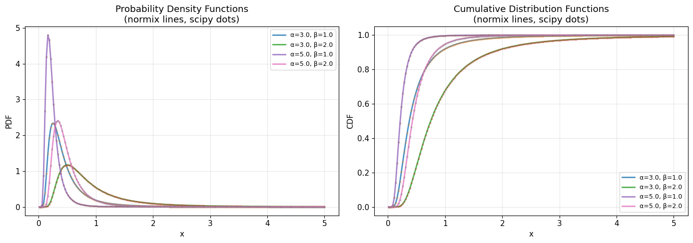
✓ normix and scipy implementations match perfectly!

3. Random Sampling and Histograms

Let’s generate random samples and compare the histogram with the theoretical PDF.

# Parameters for different distributions
test_configs = [
    {'shape': 5.0, 'rate': 2.0, 'n_samples': 10000},
    {'shape': 6.0, 'rate': 2.0, 'n_samples': 10000},
    {'shape': 7.0, 'rate': 1.0, 'n_samples': 10000},
    {'shape': 8.0, 'rate': 1.5, 'n_samples': 10000}
]

fig, axes = plt.subplots(2, 2, figsize=(14, 10))
axes = axes.flatten()

for idx, config in enumerate(test_configs):
    shape = config['shape']
    rate = config['rate']
    n_samples = config['n_samples']

    # Create distribution
    dist = InverseGamma.from_classical_params(shape=shape, rate=rate)

    # Generate samples
    samples = dist.rvs(size=n_samples, random_state=42 + idx)

    # Theoretical PDF
    x_plot = np.linspace(0.01, min(samples.max() * 1.1, 5), 200)
    pdf_theory = dist.pdf(x_plot)

    # Plot
    ax = axes[idx]
    ax.hist(samples, bins=50, density=True, alpha=0.6, color='steelblue',
            edgecolor='black', linewidth=0.5, label='Sample histogram')
    ax.plot(x_plot, pdf_theory, 'r-', linewidth=2.5, label='Theoretical PDF (normix)')

    # Also plot scipy for comparison
    scipy_dist = stats.invgamma(a=shape, scale=rate)
    scipy_pdf = scipy_dist.pdf(x_plot)
    ax.plot(x_plot, scipy_pdf, 'g--', linewidth=2, label='Scipy PDF', alpha=0.7)

    # Statistics
    sample_mean = np.mean(samples)
    theory_mean = dist.mean()
    sample_std = np.std(samples)
    theory_std = np.sqrt(dist.var())

    ax.set_xlabel('x')
    ax.set_ylabel('Density')
    ax.set_title(f'Inverse Gamma(α={shape}, β={rate})\n'
                f'Mean: {sample_mean:.3f} (theory: {theory_mean:.3f}), '
                f'Std: {sample_std:.3f} (theory: {theory_std:.3f})')
    ax.legend(loc='upper right', fontsize=9)
    ax.grid(True, alpha=0.3)

plt.tight_layout()
plt.show()

print("✓ Histograms match theoretical PDFs closely!")
print("✓ normix and scipy PDFs overlap perfectly!")

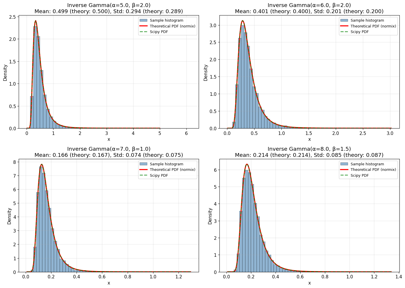
✓ Histograms match theoretical PDFs closely!
✓ normix and scipy PDFs overlap perfectly!

4. Fitting to Data

Demonstrate maximum likelihood estimation by fitting to data.

# Generate data with known parameters
true_shape = 5.0
true_rate = 2.0
n_data = 10000
data = stats.invgamma.rvs(a=true_shape, scale=true_rate, size=n_data, random_state=42)

# Fit distribution
fitted_dist = InverseGamma().fit(data)
fitted_params = fitted_dist.classical_params

print(f"Fitting {n_data} samples from InverseGamma(α={true_shape}, β={true_rate})\n")
print(f"True shape:          {true_shape:.6f}")
print(f"Fitted shape (MLE):  {fitted_params.shape:.6f}")
print(f"True rate:           {true_rate:.6f}")
print(f"Fitted rate (MLE):   {fitted_params.rate:.6f}")

# Visualize fit
fig, ax = plt.subplots(figsize=(12, 6))

# Histogram of data
ax.hist(data, bins=50, density=True, alpha=0.6, color='lightblue',
        edgecolor='black', linewidth=0.5, label='Data histogram')

# True distribution
x_plot = np.linspace(0.01, min(data.max(), 10), 200)
true_dist = InverseGamma.from_classical_params(shape=true_shape, rate=true_rate)
ax.plot(x_plot, true_dist.pdf(x_plot), 'g-', linewidth=3,
        label=f'True: α={true_shape:.1f}, β={true_rate:.1f}')

# Fitted distribution
ax.plot(x_plot, fitted_dist.pdf(x_plot), 'r--', linewidth=3,
        label=f'Fitted (normix): α={fitted_params.shape:.2f}, β={fitted_params.rate:.2f}')

ax.set_xlabel('x')
ax.set_ylabel('Density')
ax.set_title('Maximum Likelihood Estimation')
ax.legend()
ax.grid(True, alpha=0.3)

plt.tight_layout()
plt.show()

print("\n✓ MLE successfully recovers the true parameters!")

Fitting 10000 samples from InverseGamma(α=5.0, β=2.0)

True shape:          5.000000
Fitted shape (MLE):  5.099113
True rate:           2.000000
Fitted rate (MLE):   2.023664

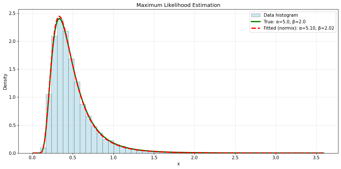
✓ MLE successfully recovers the true parameters!

fitted_params

InverseGammaParams(shape=5.099112754851492, rate=2.02366440562179)