A sample can give an accurate count of what happened while leaving the size of an unobserved loss almost unconstrained. We make this distinction precise with two laws whose samples usually coincide but whose means can be far apart. The exceedance note explains why estimating a fixed event probability does not require a moment of the underlying variable.
Use the shared notation: and are probability laws, are observations, and is a positive Pareto exponent. All draws below are iid under the chosen law.
A finite-sample indistinguishability bound¶
Let be any probability law and let , where is another law and . Define total variation by
where the supremum is over measurable events. For every integer ,
We prove this bound and its consequence for tests. To generate a sample, independently choose the component with probability at each draw. With probability , no such choice occurs and the conditional sample law is exactly . Thus for some probability law , where . For any event , the probability difference is . The union bound on the component choices gives .
More generally, a measurable test taking values in obeys
The same mixture identity proves this, because both expectations under and lie in . A test with rejection probability at most under therefore has power at most against this . Here is a test level, not the tail exponent.
A bounded law and a Pareto contamination¶
Take uniform on and an exact Pareto law with minimum and exponent . Their supports are disjoint. The event has probability zero under and under , so the total-variation bound is an equality.
For the contaminated survival and mean are
These follow by mixing the two survivals and the two finite means. For , has infinite second moment by the Pareto moment calculation, although is bounded. For any fixed , any , and any desired positive mean gap, choose , then increase until the gap is exceeded. Sample total variation stays at most . This proves that a small sample-law discrepancy need not control an unbounded mean functional over this unrestricted family.
The order of the quantifiers matters. For each fixed , the detection probability tends to one as . The construction does not say that a fixed alternative can remain hidden indefinitely.
For , , and , the mean is 300.49995 instead of 0.5, yet the probability that all observations come from is approximately 0.904833. Conditional on that event, the entire observed vector has the baseline law. The sample mean is still unbiased under : linearity gives . Rare large values supply its expectation.
What remains identifiable under additional bounds¶
If a measurable payoff satisfies with finite , the one-draw mixture identity gives
For , replace the right side by . A common payoff bound therefore changes the problem; see asymmetric payoffs. A known uniform integrability condition or a restricted parametric family can also rule out the alternatives used here. Such information is an assumption to justify.
An observation outside rejects this particular bounded exactly. For a nondegenerate Gaussian, every finite upper-tail threshold has positive exceedance probability. A large value therefore supports a statistical comparison, not a logical contradiction. No finite observation alone rejects the class of all bounded laws with unknown bounds.
Worked calculation¶
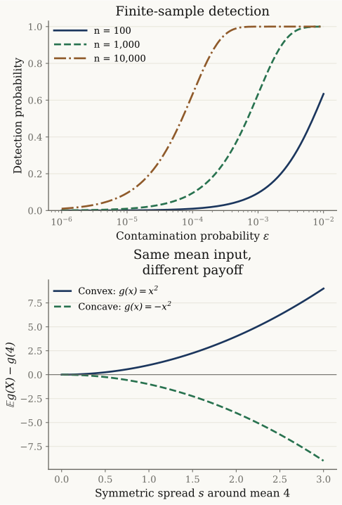
Upper panel: exact probabilities of at least one contamination, for fixed sample sizes and a varying contamination probability. These are population curves, not simulated detection rates. The lower panel is explained in the payoff note.
Use repeated_event_probability, finite_payoff_mean.
from xmath.incerto.lecture_risk import repeated_event_probability, finite_payoff_mean

epsilon, alpha, cutoff = 1e-4, 1.5, 1e6
tail_mean = alpha * cutoff / (alpha - 1)
mean = finite_payoff_mean([1 - epsilon, epsilon], [0.5, tail_mean])
print(f"Mixture mean: {mean:.4g}")
for n in (10, 1000, 10000):
    print(f"{n:d} {repeated_event_probability(epsilon, n):.3e}")
Output
Mixture mean: 300.5
10 9.996e-04
1000 9.517e-02
10000 6.321e-01
The component label is detectable here because the supports are disjoint.
Figure regeneration: uv run python demos/incerto/lecture_risk.py. The script evaluates
three sample sizes on 161 probabilities from 10-6 to 10-2 and
prints the example above. It uses no random draws or external data.
Source context¶
The chapter’s discussion motivates the inference question Taleb, 2025, ch. 3, §3.5, pp. 43–49. The mixture construction, test bound and worked example are proved here; they specify the scope in which the chapter’s inference asymmetry becomes a mathematical statement.
- Taleb, N. N. (2025). Statistical Consequences of Fat Tails (3rd ed.). https://arxiv.org/abs/2001.10488v4