This page was generated from a Jupyter notebook. You can view it on GitHub or download and run it locally.

Generalized Hyperbolic (GH) Distribution

The Generalized Hyperbolic distribution is the most general form of the normal variance-mean mixture family.

Definition

A random variable \(X\) follows a Generalized Hyperbolic distribution if it can be written as:

\[X = \mu + \gamma Y + \sqrt{Y} Z\]

where:

• \(Z \sim N(0, \Sigma)\) is independent of \(Y\)

• \(Y \sim \text{GIG}(p, a, b)\) (Generalized Inverse Gaussian)

Special Cases

Distribution	GIG Parameters	Mixing Distribution
Variance Gamma	\(b \to 0\), \(p > 0\)	Gamma\((p, a/2)\)
Normal-Inverse Gaussian	\(p = -1/2\)	InverseGaussian\((\delta, \eta)\)
Normal-Inverse Gamma	\(a \to 0\), \(p < 0\)	InverseGamma\((-p, b/2)\)
Hyperbolic	\(p = 1\)	GIG\((1, a, b)\)

Key Properties

• Joint distribution \(f(x, y)\) is an exponential family

• Marginal distribution \(f(x)\) is NOT an exponential family

• Fitting uses the EM algorithm with parameter regularization

import numpy as np
import matplotlib.pyplot as plt
from matplotlib.gridspec import GridSpec
from scipy import stats

from normix.distributions.mixtures import (
    GeneralizedHyperbolic, JointGeneralizedHyperbolic,
    VarianceGamma, NormalInverseGaussian, NormalInverseGamma
)
from normix.utils import (
    plot_joint_distribution_1d, plot_marginal_distribution_2d,
    validate_moments, print_moment_validation,
    fit_and_track_convergence, plot_em_convergence,
    test_joint_fitting, print_fitting_results
)

plt.style.use('seaborn-v0_8-whitegrid')
%matplotlib inline

print("Imports successful!")

Imports successful!

---

1. Joint Distribution: \(f(x, y)\) (Exponential Family)

The joint distribution is:

\[f(x, y) = f(x|y) \cdot f(y)\]

where:

• \(X|Y \sim N(\mu + \gamma Y, \Sigma Y)\)

• \(Y \sim \text{GIG}(p, a, b)\)

# Define parameters for 1D joint distribution
params_1d = {
    'mu': np.array([0.0]),
    'gamma': np.array([0.5]),
    'sigma': np.array([[1.0]]),
    'p': 1.0,
    'a': 1.0,
    'b': 1.0
}

# Create joint distribution
jgh_1d = JointGeneralizedHyperbolic.from_classical_params(**params_1d)
print("Created:", jgh_1d)
print("\nClassical parameters:", jgh_1d.classical_params)

Created: JointGeneralizedHyperbolic(μ=0.000, γ=0.500, p=1.000, a=1.000, b=1.000)

Classical parameters: GHParams(mu=array([0.]), gamma=array([0.5]), sigma=array([[1.]]), p=np.float64(1.0), a=np.float64(1.0), b=np.float64(1.0))

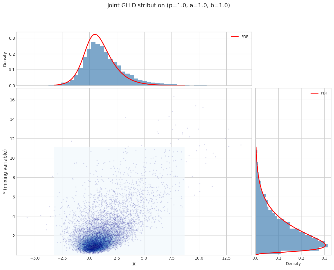
# Visualize joint distribution
fig = plot_joint_distribution_1d(
    jgh_1d, n_samples=5000, random_state=42,
    title=f"Joint GH Distribution (p={params_1d['p']}, a={params_1d['a']}, b={params_1d['b']})"
)
plt.tight_layout()
plt.show()

/tmp/ipykernel_2346057/2167798511.py:6: UserWarning: This figure includes Axes that are not compatible with tight_layout, so results might be incorrect.
  plt.tight_layout()

1.1 Moment Validation

# Validate moments
moment_results = validate_moments(jgh_1d, n_samples=20000, random_state=42, is_joint=True)
print_moment_validation(moment_results)

============================================================
Moment Validation: Distribution
============================================================
X_mean    : sample =     1.3374, theory =     1.3497, rel_err = 9.18e-03
Y_mean    : sample =     2.7129, theory =     2.6995, rel_err = 4.98e-03
X_var     : sample =     3.8364, theory =     3.8272, rel_err = 2.43e-03
Y_var     : sample =     4.5105, theory =     4.5107, rel_err = 5.71e-05

1.2 MLE Fitting (Complete Data)

# Test MLE fitting for joint distribution
fitted_dist, fitted_params, param_errors = test_joint_fitting(
    JointGeneralizedHyperbolic,
    params_1d,
    n_samples=10000,
    random_state=42
)
print_fitting_results(params_1d, fitted_params, param_errors, name="JointGH")

============================================================
Fitting Results: JointGH
============================================================
Parameter                  True          Fitted    Rel.Error
------------------------------------------------------------
mu                       0.0000         -0.0110     1.10e+08
gamma                    0.5000          0.5025     5.00e-03
sigma                    1.0000          1.0071     7.11e-03
p                        1.0000          0.9702     2.98e-02
a                        1.0000          0.9982     1.76e-03
b                        1.0000          1.0471     4.71e-02

---

2. Marginal Distribution: \(f(x)\) (2D Case)

The marginal distribution is NOT an exponential family.

# Define 2D marginal distribution parameters
params_2d = {
    'mu': np.array([0.0, 0.0]),
    'gamma': np.array([0.5, -0.3]),
    'sigma': np.array([[1.0, 0.3], [0.3, 1.0]]),
    'p': 1.0,
    'a': 1.0,
    'b': 1.0
}

# Create marginal distribution
gh_2d = GeneralizedHyperbolic.from_classical_params(**params_2d)
print("Created:", gh_2d)

Created: GeneralizedHyperbolic(d=2, p=1.000, a=1.000, b=1.000)

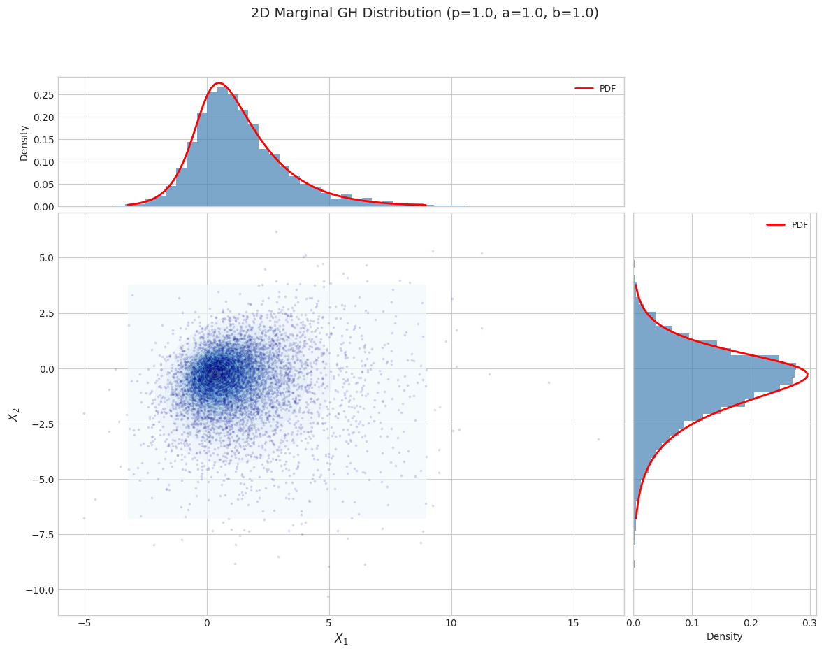
# Visualize 2D marginal distribution
fig = plot_marginal_distribution_2d(
    gh_2d, n_samples=5000, random_state=42,
    title=f"2D Marginal GH Distribution (p={params_2d['p']}, a={params_2d['a']}, b={params_2d['b']})"
)
plt.tight_layout()
plt.show()

/tmp/ipykernel_2346057/2887610028.py:6: UserWarning: This figure includes Axes that are not compatible with tight_layout, so results might be incorrect.
  plt.tight_layout()

2.1 EM Algorithm Fitting

The marginal distribution requires the EM algorithm for fitting.

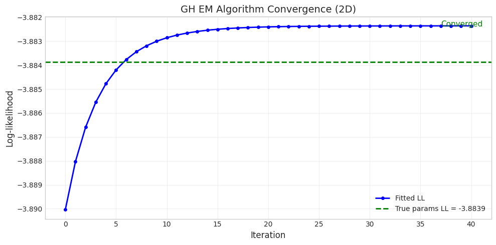
# Generate data from true distribution
true_gh = GeneralizedHyperbolic.from_classical_params(**params_2d)
X_data = true_gh.rvs(size=5000, random_state=42)

# Compute true log-likelihood for reference
true_ll = np.mean(true_gh.logpdf(X_data))
print(f"True parameters log-likelihood: {true_ll:.4f}")

# Fit using EM algorithm with regularization
print("\nFitting with EM algorithm (det_sigma_one regularization)...")
fitted_gh, convergence = fit_and_track_convergence(
    GeneralizedHyperbolic,
    X_data,
    max_iter=100,
    tol=1e-2,  # Use reasonable tolerance for GH
    regularization='det_sigma_one',
)

print(f"\nConverged: {convergence.converged}")
print(f"Final log-likelihood: {convergence.log_likelihoods[-1]:.4f}")
print(f"Improvement over true: {convergence.log_likelihoods[-1] - true_ll:.4f}")

True parameters log-likelihood: -3.8839

Fitting with EM algorithm (det_sigma_one regularization)...

Converged: True
Final log-likelihood: -3.8824
Improvement over true: 0.0015

# Plot convergence with true log-likelihood reference
fig = plot_em_convergence(
    convergence,
    title="GH EM Algorithm Convergence (2D)",
    true_ll=true_ll
)
plt.show()

---

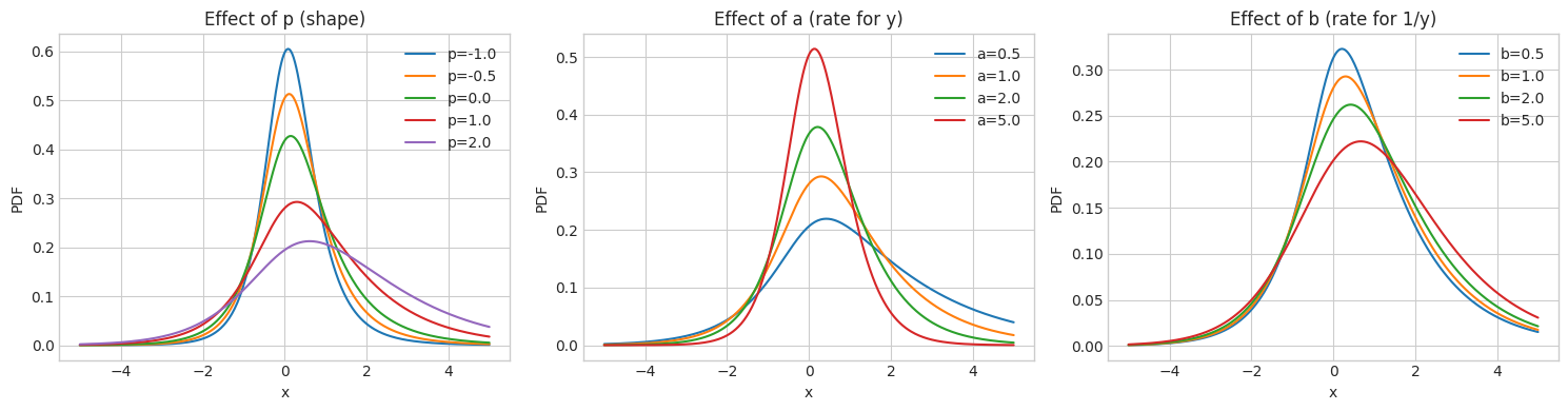
3. Effect of GIG Parameters

The GIG parameters \((p, a, b)\) control the shape of the mixing distribution and thus the behavior of the GH distribution.

fig, axes = plt.subplots(1, 3, figsize=(15, 4))

# Base parameters
base_mu = np.array([0.0])
base_gamma = np.array([0.3])
base_sigma = np.array([[1.0]])

x = np.linspace(-5, 5, 300)

# Effect of p
ax = axes[0]
for p in [-1.0, -0.5, 0.0, 1.0, 2.0]:
    try:
        gh = GeneralizedHyperbolic.from_classical_params(
            mu=base_mu, gamma=base_gamma, sigma=base_sigma, p=p, a=1.0, b=1.0
        )
        pdf = np.array([gh.pdf(np.array([xi])) for xi in x])
        ax.plot(x, pdf, label=f'p={p}')
    except:
        pass
ax.set_title('Effect of p (shape)')
ax.set_xlabel('x')
ax.set_ylabel('PDF')
ax.legend()

# Effect of a
ax = axes[1]
for a in [0.5, 1.0, 2.0, 5.0]:
    try:
        gh = GeneralizedHyperbolic.from_classical_params(
            mu=base_mu, gamma=base_gamma, sigma=base_sigma, p=1.0, a=a, b=1.0
        )
        pdf = np.array([gh.pdf(np.array([xi])) for xi in x])
        ax.plot(x, pdf, label=f'a={a}')
    except:
        pass
ax.set_title('Effect of a (rate for y)')
ax.set_xlabel('x')
ax.set_ylabel('PDF')
ax.legend()

# Effect of b
ax = axes[2]
for b in [0.5, 1.0, 2.0, 5.0]:
    try:
        gh = GeneralizedHyperbolic.from_classical_params(
            mu=base_mu, gamma=base_gamma, sigma=base_sigma, p=1.0, a=1.0, b=b
        )
        pdf = np.array([gh.pdf(np.array([xi])) for xi in x])
        ax.plot(x, pdf, label=f'b={b}')
    except:
        pass
ax.set_title('Effect of b (rate for 1/y)')
ax.set_xlabel('x')
ax.set_ylabel('PDF')
ax.legend()

plt.tight_layout()
plt.show()

---

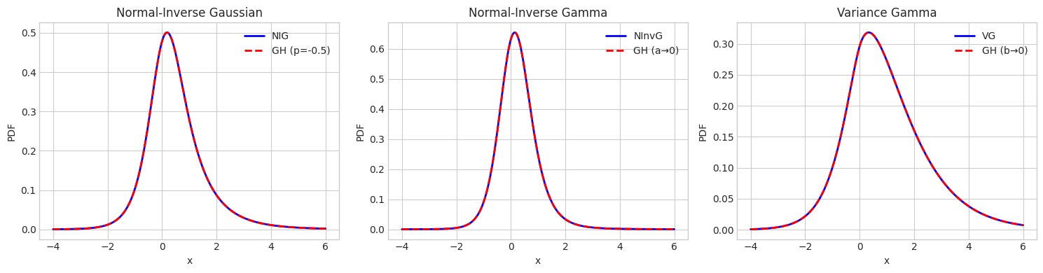
4. Special Case Comparison

Verify that GH special cases match their dedicated implementations.

# Test parameters
mu = np.array([0.0])
gamma = np.array([0.5])
sigma = np.array([[1.0]])

x = np.linspace(-4, 6, 300)

fig, axes = plt.subplots(1, 3, figsize=(15, 4))

# NIG comparison (p = -0.5)
ax = axes[0]
nig_params = {'delta': 1.0, 'eta': 1.0}
nig = NormalInverseGaussian.from_classical_params(mu=mu, gamma=gamma, sigma=sigma, **nig_params)
gh_nig = GeneralizedHyperbolic.as_normal_inverse_gaussian(mu=mu, gamma=gamma, sigma=sigma, **nig_params)

nig_pdf = np.array([nig.pdf(np.array([xi])) for xi in x])
gh_nig_pdf = np.array([gh_nig.pdf(np.array([xi])) for xi in x])

ax.plot(x, nig_pdf, 'b-', linewidth=2, label='NIG')
ax.plot(x, gh_nig_pdf, 'r--', linewidth=2, label='GH (p=-0.5)')
ax.set_title('Normal-Inverse Gaussian')
ax.set_xlabel('x')
ax.set_ylabel('PDF')
ax.legend()
print(f"NIG mean: {nig.mean()}, GH mean: {gh_nig.mean()}")

# NInvG comparison (a → 0)
ax = axes[1]
ninvg_params = {'shape': 3.0, 'rate': 1.0}
ninvg = NormalInverseGamma.from_classical_params(mu=mu, gamma=gamma, sigma=sigma, **ninvg_params)
gh_ninvg = GeneralizedHyperbolic.as_normal_inverse_gamma(mu=mu, gamma=gamma, sigma=sigma, **ninvg_params)

ninvg_pdf = np.array([ninvg.pdf(np.array([xi])) for xi in x])
gh_ninvg_pdf = np.array([gh_ninvg.pdf(np.array([xi])) for xi in x])

ax.plot(x, ninvg_pdf, 'b-', linewidth=2, label='NInvG')
ax.plot(x, gh_ninvg_pdf, 'r--', linewidth=2, label='GH (a→0)')
ax.set_title('Normal-Inverse Gamma')
ax.set_xlabel('x')
ax.set_ylabel('PDF')
ax.legend()
print(f"NInvG mean: {ninvg.mean()}, GH mean: {gh_ninvg.mean()}")

# VG comparison (b → 0)
ax = axes[2]
vg_params = {'shape': 2.0, 'rate': 1.0}
vg = VarianceGamma.from_classical_params(mu=mu, gamma=gamma, sigma=sigma, **vg_params)
gh_vg = GeneralizedHyperbolic.as_variance_gamma(mu=mu, gamma=gamma, sigma=sigma, **vg_params)

vg_pdf = np.array([vg.pdf(np.array([xi])) for xi in x])
gh_vg_pdf = np.array([gh_vg.pdf(np.array([xi])) for xi in x])

ax.plot(x, vg_pdf, 'b-', linewidth=2, label='VG')
ax.plot(x, gh_vg_pdf, 'r--', linewidth=2, label='GH (b→0)')
ax.set_title('Variance Gamma')
ax.set_xlabel('x')
ax.set_ylabel('PDF')
ax.legend()
print(f"VG mean: {vg.mean()}, GH mean: {gh_vg.mean()}")

plt.tight_layout()
plt.show()

NIG mean: [0.5], GH mean: [0.5]
NInvG mean: [0.25], GH mean: [0.25]
VG mean: [1.], GH mean: [1.]

---

5. Parameter Regularization

The GH model is not identifiable since \((\mu, \gamma/c, \Sigma/c, p, cb, a/c)\) gives the same distribution for any \(c > 0\).

Available regularization methods:

• det_sigma_one: Fix \(|\Sigma| = 1\) (recommended)

• sigma_diagonal_one: Fix \(\Sigma_{11} = 1\)

• fix_p: Fix \(p\) to a specific value

• none: No regularization

from normix.distributions.mixtures import REGULARIZATION_METHODS

print("Available regularization methods:")
for name in REGULARIZATION_METHODS:
    print(f"  - {name}")

Available regularization methods:
  - det_sigma_one
  - sigma_diagonal_one
  - fix_p
  - none

# Compare different regularizations
X_data = true_gh.rvs(size=3000, random_state=42)

regularizations = ['det_sigma_one', 'fix_p']
results = {}

for reg in regularizations:
    print(f"\n--- Regularization: {reg} ---")
    fitted = GeneralizedHyperbolic()
    kwargs = {'regularization': reg}
    if reg == 'fix_p':
        kwargs['regularization_params'] = {'p_fixed': 1.0}

    fitted.fit(X_data, max_iter=30, verbose=0, **kwargs)
    params = fitted.classical_params

    print(f"  p = {params.p:.4f}")
    print(f"  a = {params.a:.4f}")
    print(f"  b = {params.b:.4f}")
    print(f"  |Σ| = {np.linalg.det(params.sigma):.4f}")
    print(f"  Mean = {fitted.mean()}")
    results[reg] = fitted

--- Regularization: det_sigma_one ---
  p = 0.5896
  a = 0.9347
  b = 1.6064
  |Σ| = 1.0000
  Mean = [ 1.27654667 -0.82581383]

--- Regularization: fix_p ---
  p = 1.0000
  a = 0.3575
  b = 14.3831
  |Σ| = 0.0738
  Mean = [ 1.58034717 -1.01797886]

---

6. Exponential Family Structure

The joint distribution is an exponential family with:

Sufficient statistics:

\[t(x, y) = [\log y, y^{-1}, y, x, xy^{-1}, \text{vec}(xx^T y^{-1})]\]

Natural parameters:

\[\theta = [p - 1 - d/2, -(b + \frac{1}{2}\mu^T\Lambda\mu), -(a + \frac{1}{2}\gamma^T\Lambda\gamma), \Lambda\gamma, \Lambda\mu, -\frac{1}{2}\text{vec}(\Lambda)]\]

# Show parameter conversions
print("=== Exponential Family Parameters ===")
print(f"\nClassical: {jgh_1d.classical_params}")
print(f"\nNatural: {jgh_1d.natural_params}")
print(f"\nExpectation: {jgh_1d.expectation_params[:6]}...")  # First 6 components

=== Exponential Family Parameters ===

Classical: GHParams(mu=array([0.]), gamma=array([0.5]), sigma=array([[1.]]), p=np.float64(1.0), a=np.float64(1.0), b=np.float64(1.0))

Natural: [-0.5   -1.    -1.125  0.5    0.    -0.5  ]

Expectation: [0.69948394 0.69948394 2.69948394 1.34974197 0.5        1.67487098]...

# Verify sufficient statistics match expectation parameters
n_samples = 20000
X, Y = jgh_1d.rvs(size=n_samples, random_state=42)
t_samples = jgh_1d._sufficient_statistics(X, Y)
eta_sample = np.mean(t_samples, axis=0)
eta_theory = jgh_1d.expectation_params

print("E[t(X,Y)] from samples vs theoretical:")
print(f"  E[log Y]:     {eta_sample[0]:.4f} vs {eta_theory[0]:.4f}")
print(f"  E[1/Y]:       {eta_sample[1]:.4f} vs {eta_theory[1]:.4f}")
print(f"  E[Y]:         {eta_sample[2]:.4f} vs {eta_theory[2]:.4f}")

E[t(X,Y)] from samples vs theoretical:
  E[log Y]:     0.7052 vs 0.6995
  E[1/Y]:       0.6942 vs 0.6995
  E[Y]:         2.7129 vs 2.6995

---

Summary

The Generalized Hyperbolic distribution:

1. Most general normal variance-mean mixture

2. Joint distribution is an exponential family

3. Marginal distribution requires EM algorithm for fitting

4. Special cases include VG, NIG, NInvG, and more

5. Regularization is needed due to identifiability issues