This page was generated from a Jupyter notebook. You can view it on GitHub or download and run it locally.
S&P 500 Stocks Multivariate Empirical Study
This notebook compares multivariate probability distributions for modeling S&P 500 stock returns. The main purpose is to test the EM algorithm in real-world high-dimensional settings.
Distributions Compared
Multivariate Normal - Baseline Gaussian distribution
Variance Gamma (VG) - Normal-Gamma mixture, semi-heavy tails
Normal Inverse Gamma (NInvG) - Normal-InverseGamma mixture, heavy tails
Normal Inverse Gaussian (NIG) - Normal-InverseGaussian mixture
Generalized Hyperbolic (GH) - Most general, encompasses VG, NInvG, NIG as special cases
Methodology
Data: 10 years of S&P 500 constituent stocks daily returns
Training: First 5 years (in-sample)
Testing: Last 5 years (out-of-sample)
EM Algorithm: Track convergence and timing in high dimensions
Testing Methods: Random portfolio projections, KS/AD tests, QQ plots
Parameter Analysis: Compare location (μ) vs skewness (γ) parameters across stocks
[1]:
import numpy as np
import pandas as pd
import matplotlib.pyplot as plt
from matplotlib.gridspec import GridSpec
from scipy import stats
from scipy.stats import ks_2samp, anderson_ksamp
import warnings
import time
warnings.filterwarnings('ignore')

# Import normix distributions
from normix.distributions.multivariate import MultivariateNormal
from normix.distributions.mixtures import (
    VarianceGamma, NormalInverseGamma, NormalInverseGaussian, GeneralizedHyperbolic
)

plt.style.use('seaborn-v0_8-whitegrid')
%matplotlib inline

print("Imports successful!")
Imports successful!
1. Load S&P 500 Stock Returns Data
The log returns data is pre-computed and stored in data/sp500_returns.csv. This file is generated by scripts/download_sp500_data.py which fetches S&P 500 constituent stocks from Wikipedia and downloads historical price data from Yahoo Finance.
[2]:
# Load pre-computed log returns from CSV
import os

data_path = '../data/sp500_returns.csv'

if not os.path.exists(data_path):
    raise FileNotFoundError(
        f"Data file not found at {data_path}. "
        "Please run 'python scripts/download_sp500_data.py' first to generate the data."
    )

log_returns = pd.read_csv(data_path, index_col='Date', parse_dates=True)

print(f"Loaded log returns from: {data_path}")
print(f"Shape: {log_returns.shape}")
print(f"Date range: {log_returns.index[0].date()} to {log_returns.index[-1].date()}")
print(f"Number of stocks: {len(log_returns.columns)}")
print(f"First 10 tickers: {list(log_returns.columns[:10])}")
Loaded log returns from: ../data/sp500_returns.csv
Shape: (2551, 224)
Date range: 2015-12-10 to 2026-02-03
Number of stocks: 224
First 10 tickers: ['A', 'AAPL', 'ABBV', 'ABT', 'ACN', 'ADBE', 'ADI', 'AEP', 'AES', 'AIG']
[3]:
# Use ALL stocks from the CSV file (no filtering needed - data is already clean)
# Note: High-dimensional fitting can be slow - adjust MAX_STOCKS if needed for computational constraints
MAX_STOCKS = None  # Set to a number (e.g., 100) to limit, or None for all available stocks

# Select all stocks, sorted alphabetically
all_tickers = sorted(log_returns.columns.tolist())

if MAX_STOCKS is not None and MAX_STOCKS < len(all_tickers):
    selected_tickers = all_tickers[:MAX_STOCKS]
    print(f"Limited to {MAX_STOCKS} stocks for computational efficiency")
else:
    selected_tickers = all_tickers

log_returns_selected = log_returns[selected_tickers]

print(f"Selected {len(selected_tickers)} stocks for analysis:")
print(f"Tickers: {selected_tickers[:20]}{'...' if len(selected_tickers) > 20 else ''}")
Selected 224 stocks for analysis:
Tickers: ['A', 'AAPL', 'ABBV', 'ABT', 'ACN', 'ADBE', 'ADI', 'AEP', 'AES', 'AIG', 'ALL', 'AMAT', 'AMD', 'AMGN', 'AMT', 'AMZN', 'APA', 'APD', 'ARE', 'AVB']...
[4]:
# Split into training (first half) and testing (second half)
n_total = len(log_returns_selected)
n_train = n_total // 2

train_df = log_returns_selected.iloc[:n_train]
test_df = log_returns_selected.iloc[n_train:]

# Convert to numpy arrays
returns_train = train_df.values
returns_test = test_df.values

print(f"\nTraining period: {train_df.index[0].date()} to {train_df.index[-1].date()}")
print(f"Training samples: {returns_train.shape[0]}, dimensions: {returns_train.shape[1]}")
print(f"\nTesting period: {test_df.index[0].date()} to {test_df.index[-1].date()}")
print(f"Testing samples: {returns_test.shape[0]}, dimensions: {returns_test.shape[1]}")
Training period: 2015-12-10 to 2021-01-04
Training samples: 1275, dimensions: 224

Testing period: 2021-01-05 to 2026-02-03
Testing samples: 1276, dimensions: 224
[5]:
# Display training data statistics
print("--- Training Data Statistics ---")
mean_returns = returns_train.mean(axis=0) * 100
std_returns = returns_train.std(axis=0) * 100
skewness = stats.skew(returns_train, axis=0)
kurtosis = stats.kurtosis(returns_train, axis=0)

stats_df = pd.DataFrame({
    'Mean (%)': mean_returns,
    'Std (%)': std_returns,
    'Skewness': skewness,
    'Kurtosis': kurtosis
}, index=selected_tickers)

print(stats_df.round(4))

print(f"\n--- Summary ---")
print(f"Average mean return: {mean_returns.mean():.4f}%")
print(f"Average volatility: {std_returns.mean():.4f}%")
print(f"Average skewness: {skewness.mean():.4f}")
print(f"Average excess kurtosis: {kurtosis.mean():.4f}")
--- Training Data Statistics ---
      Mean (%)  Std (%)  Skewness  Kurtosis
A       0.0872   1.6669   -0.6919    7.1136
AAPL    0.1236   1.8991   -0.3552    7.4072
ABBV    0.0669   1.8452   -1.0039   14.5807
ABT     0.0772   1.5974   -0.3903    7.7395
ACN     0.0751   1.5903   -0.0063    8.8244
...        ...      ...       ...       ...
WMB    -0.0040   3.1997   -1.8227   39.9337
WMT     0.0801   1.3877    0.7979   15.6157
XEL     0.0612   1.4044   -1.0123   19.8592
XOM    -0.0285   1.8035   -0.1616   10.5633
ZBH     0.0368   1.8834   -0.1455   12.3800

[224 rows x 4 columns]

--- Summary ---
Average mean return: 0.0523%
Average volatility: 1.9748%
Average skewness: -0.5328
Average excess kurtosis: 17.8969
2. Fit Distributions with EM Algorithm Tracking
[6]:
# Storage for fitted distributions and convergence info
fitted_dists = {}
fitting_times = {}
convergence_history = {}

d = returns_train.shape[1]  # dimension
print(f"Fitting distributions to {d}-dimensional data...")
Fitting distributions to 224-dimensional data...
2.1 Multivariate Normal (Baseline)
[7]:
print("Fitting Multivariate Normal...")
start_time = time.time()

mvn = MultivariateNormal(d=d).fit(returns_train)

fitting_times['MVN'] = time.time() - start_time
fitted_dists['MVN'] = mvn

print(f"Fitting time: {fitting_times['MVN']:.2f}s")
print(f"Mean log-likelihood (train): {np.mean(mvn.logpdf(returns_train)):.4f}")
print(f"Mean log-likelihood (test): {np.mean(mvn.logpdf(returns_test)):.4f}")
Fitting Multivariate Normal...
Fitting time: 0.08s
Mean log-likelihood (train): 702.2173
Mean log-likelihood (test): 624.0910
2.2 Variance Gamma (VG)
[8]:
print("Fitting Variance Gamma...")
start_time = time.time()

# Create a custom verbose fit to track convergence
vg = VarianceGamma()
vg_ll_history = []

# We'll manually track convergence by fitting with verbose=2
# and capturing the output, or by modifying the fit loop
# For simplicity, just fit with verbose
vg.fit(returns_train, max_iter=100, tol=1e-3, verbose=1)

fitting_times['VG'] = time.time() - start_time
fitted_dists['VG'] = vg

print(f"\nFitting time: {fitting_times['VG']:.2f}s")
print(f"Mean log-likelihood (train): {np.mean(vg.logpdf(returns_train)):.4f}")
print(f"Mean log-likelihood (test): {np.mean(vg.logpdf(returns_test)):.4f}")
Fitting Variance Gamma...
Initial log-likelihood: 445.622318
Iteration 1: log-likelihood = 702.301546
Iteration 2: log-likelihood = 712.297042
Iteration 3: log-likelihood = 718.818670
Iteration 4: log-likelihood = 720.217824
Iteration 5: log-likelihood = 720.394836
Iteration 6: log-likelihood = 720.414506
Iteration 7: log-likelihood = 720.416618
Iteration 8: log-likelihood = 720.416843
Iteration 9: log-likelihood = 720.416867
Iteration 10: log-likelihood = 720.416869
Converged at iteration 10
Final log-likelihood: 720.416869

Fitting time: 2.68s
Mean log-likelihood (train): 720.4169
Mean log-likelihood (test): 666.1294
2.3 Normal Inverse Gamma (NInvG)
[9]:
print("Fitting Normal Inverse Gamma...")
start_time = time.time()

ninvg = NormalInverseGamma()
ninvg.fit(returns_train, max_iter=100, tol=1e-3, verbose=1)

fitting_times['NInvG'] = time.time() - start_time
fitted_dists['NInvG'] = ninvg

print(f"\nFitting time: {fitting_times['NInvG']:.2f}s")
print(f"Mean log-likelihood (train): {np.mean(ninvg.logpdf(returns_train)):.4f}")
print(f"Mean log-likelihood (test): {np.mean(ninvg.logpdf(returns_test)):.4f}")
Fitting Normal Inverse Gamma...
Initial log-likelihood: 667.849344
Iteration 1: log-likelihood = 714.870073
Iteration 2: log-likelihood = 720.056497
Iteration 3: log-likelihood = 720.590019
Iteration 4: log-likelihood = 720.629384
Iteration 5: log-likelihood = 720.632118
Iteration 6: log-likelihood = 720.632313
Iteration 7: log-likelihood = 720.632327
Iteration 8: log-likelihood = 720.632328
Converged at iteration 8
Final log-likelihood: 720.632328

Fitting time: 0.21s
Mean log-likelihood (train): 720.6323
Mean log-likelihood (test): 666.0525
2.4 Normal Inverse Gaussian (NIG)
[10]:
print("Fitting Normal Inverse Gaussian...")
start_time = time.time()

nig = NormalInverseGaussian()
nig.fit(returns_train, max_iter=100, tol=1e-3, verbose=1)

fitting_times['NIG'] = time.time() - start_time
fitted_dists['NIG'] = nig

print(f"\nFitting time: {fitting_times['NIG']:.2f}s")
print(f"Mean log-likelihood (train): {np.mean(nig.logpdf(returns_train)):.4f}")
print(f"Mean log-likelihood (test): {np.mean(nig.logpdf(returns_test)):.4f}")
Fitting Normal Inverse Gaussian...
Initial log-likelihood: 529.719043
Iteration 1: log-likelihood = 706.340524
Iteration 2: log-likelihood = 718.128162
Iteration 3: log-likelihood = 720.312762
Iteration 4: log-likelihood = 720.540481
Iteration 5: log-likelihood = 720.560807
Iteration 6: log-likelihood = 720.562597
Iteration 7: log-likelihood = 720.562757
Iteration 8: log-likelihood = 720.562771
Iteration 9: log-likelihood = 720.562772
Converged at iteration 9
Final log-likelihood: 720.562772

Fitting time: 2.48s
Mean log-likelihood (train): 720.5628
Mean log-likelihood (test): 666.1407
2.5 Generalized Hyperbolic (GH)
[11]:
print("Fitting Generalized Hyperbolic...")
print("This is the most general model and may take longer...")
start_time = time.time()

gh = GeneralizedHyperbolic()
gh.fit(returns_train, max_iter=100, tol=1e-3, verbose=1, regularization='det_sigma_one')

fitting_times['GH'] = time.time() - start_time
fitted_dists['GH'] = gh

print(f"\nFitting time: {fitting_times['GH']:.2f}s")
print(f"Mean log-likelihood (train): {np.mean(gh.logpdf(returns_train)):.4f}")
print(f"Mean log-likelihood (test): {np.mean(gh.logpdf(returns_test)):.4f}")
Fitting Generalized Hyperbolic...
This is the most general model and may take longer...
Initial log-likelihood: 720.560807
Iteration 1: log-likelihood = 720.562228
Iteration 2: log-likelihood = 720.562318
Iteration 3: log-likelihood = 720.562324
Iteration 4: log-likelihood = 720.562325
Converged

Fitting time: 3.60s
Mean log-likelihood (train): 720.5623
Mean log-likelihood (test): 666.1362
3. Summary of Fitting Results
[12]:
# Compute log-likelihoods for all distributions
results = []

for name, dist in fitted_dists.items():
    train_ll = np.mean(dist.logpdf(returns_train))
    test_ll = np.mean(dist.logpdf(returns_test))

    results.append({
        'Distribution': name,
        'Train LL': train_ll,
        'Test LL': test_ll,
        'Fitting Time (s)': fitting_times[name]
    })

results_df = pd.DataFrame(results)
results_df = results_df.sort_values('Test LL', ascending=False)

print("\n" + "="*70)
print("SUMMARY: Distribution Fitting Results")
print("="*70)
print(results_df.to_string(index=False))
print("="*70)
======================================================================
SUMMARY: Distribution Fitting Results
======================================================================
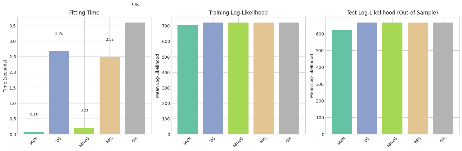
Distribution Train LL Test LL Fitting Time (s)
NIG 720.562772 666.140655 2.481778
GH 720.562325 666.136179 3.599135
VG 720.416869 666.129448 2.676722
NInvG 720.632328 666.052491 0.207242
MVN 702.217252 624.090997 0.076318
======================================================================
[13]:
# Visualization of fitting times and log-likelihoods
fig, axes = plt.subplots(1, 3, figsize=(15, 5))

dist_names = list(fitted_dists.keys())
colors = plt.cm.Set2(np.linspace(0, 1, len(dist_names)))

# Plot 1: Fitting times
ax1 = axes[0]
times = [fitting_times[n] for n in dist_names]
bars1 = ax1.bar(dist_names, times, color=colors)
ax1.set_ylabel('Time (seconds)')
ax1.set_title('Fitting Time')
ax1.tick_params(axis='x', rotation=45)

# Add value labels
for bar, t in zip(bars1, times):
    ax1.text(bar.get_x() + bar.get_width()/2, bar.get_height() + 0.5,
             f'{t:.1f}s', ha='center', va='bottom', fontsize=9)

# Plot 2: Train log-likelihood
ax2 = axes[1]
train_lls = [np.mean(fitted_dists[n].logpdf(returns_train)) for n in dist_names]
bars2 = ax2.bar(dist_names, train_lls, color=colors)
ax2.set_ylabel('Mean Log-Likelihood')
ax2.set_title('Training Log-Likelihood')
ax2.tick_params(axis='x', rotation=45)

# Plot 3: Test log-likelihood
ax3 = axes[2]
test_lls = [np.mean(fitted_dists[n].logpdf(returns_test)) for n in dist_names]
bars3 = ax3.bar(dist_names, test_lls, color=colors)
ax3.set_ylabel('Mean Log-Likelihood')
ax3.set_title('Test Log-Likelihood (Out-of-Sample)')
ax3.tick_params(axis='x', rotation=45)

plt.tight_layout()
plt.savefig('fitting_summary.png', dpi=150, bbox_inches='tight')
plt.show()
4. Random Portfolio Projections Testing
To test multivariate distributions, we use random portfolio projections:
Generate random weight vectors
Project returns onto 1D using these weights
Compare simulated samples from fitted distributions vs actual test data
Use KS and Anderson-Darling tests
[14]:
def generate_random_weights(d, n_portfolios=100, random_state=None):
    """
    Generate random portfolio weights.

    Parameters
    ----------
    d : int
        Number of assets.
    n_portfolios : int
        Number of random portfolios to generate.
    random_state : int, optional
        Random seed.

    Returns
    -------
    weights : ndarray
        Shape (n_portfolios, d), each row sums to 1.
    """
    rng = np.random.default_rng(random_state)

    # Generate random weights from Dirichlet distribution (uniform on simplex)
    # This ensures weights are positive and sum to 1
    weights = rng.dirichlet(np.ones(d), size=n_portfolios)

    return weights


def project_returns(returns, weights):
    """
    Project multivariate returns to 1D portfolio returns.

    Parameters
    ----------
    returns : ndarray
        Shape (n_samples, d).
    weights : ndarray
        Shape (n_portfolios, d) or (d,).

    Returns
    -------
    portfolio_returns : ndarray
        Shape (n_samples, n_portfolios) or (n_samples,).
    """
    if weights.ndim == 1:
        return returns @ weights
    else:
        return returns @ weights.T
[15]:
# Generate random portfolios
N_PORTFOLIOS = 100
random_weights = generate_random_weights(d, n_portfolios=N_PORTFOLIOS, random_state=42)

print(f"Generated {N_PORTFOLIOS} random portfolios")
print(f"Weight matrix shape: {random_weights.shape}")
print(f"First portfolio weights: {random_weights[0][:5].round(3)}...")
Generated 100 random portfolios
Weight matrix shape: (100, 224)
First portfolio weights: [0.011 0.011 0.011 0.001 0.   ]...
[16]:
def portfolio_test(dist, returns_test, weights, n_samples=10000, random_state=None):
    """
    Test a distribution using random portfolio projections.

    Parameters
    ----------
    dist : distribution object
        Fitted distribution.
    returns_test : ndarray
        Test data, shape (n_test, d).
    weights : ndarray
        Portfolio weights, shape (n_portfolios, d).
    n_samples : int
        Number of samples to generate from distribution.
    random_state : int, optional
        Random seed.

    Returns
    -------
    results : dict
        Dictionary with KS and AD test statistics.
    """
    # Generate samples from fitted distribution
    samples = dist.rvs(size=n_samples, random_state=random_state)

    n_portfolios = weights.shape[0]
    ks_stats = []
    ks_pvals = []
    ad_stats = []

    for i in range(n_portfolios):
        w = weights[i]

        # Project to 1D
        test_proj = returns_test @ w
        sample_proj = samples @ w

        # KS test
        ks_stat, ks_pval = ks_2samp(test_proj, sample_proj)
        ks_stats.append(ks_stat)
        ks_pvals.append(ks_pval)

        # Anderson-Darling test (two-sample)
        try:
            ad_result = anderson_ksamp([test_proj, sample_proj])
            ad_stats.append(ad_result.statistic)
        except Exception:
            ad_stats.append(np.nan)

    return {
        'ks_stats': np.array(ks_stats),
        'ks_pvals': np.array(ks_pvals),
        'ad_stats': np.array(ad_stats),
        'ks_mean': np.mean(ks_stats),
        'ks_median': np.median(ks_stats),
        'ad_mean': np.nanmean(ad_stats),
        'ad_median': np.nanmedian(ad_stats),
        'ks_reject_rate': np.mean(np.array(ks_pvals) < 0.05)  # Rejection rate at 5%
    }
[17]:
# Run portfolio tests for all distributions
portfolio_results = {}

print("Running portfolio projection tests...")
print(f"Testing with {N_PORTFOLIOS} random portfolios\n")

for name, dist in fitted_dists.items():
    print(f"Testing {name}...")
    try:
        results = portfolio_test(dist, returns_test, random_weights,
                                 n_samples=5000, random_state=42)
        portfolio_results[name] = results
        print(f"  KS mean: {results['ks_mean']:.4f}, KS reject rate: {results['ks_reject_rate']:.2%}")
        print(f"  AD mean: {results['ad_mean']:.4f}")
    except Exception as e:
        print(f"  Error: {e}")
        portfolio_results[name] = None
Running portfolio projection tests...
Testing with 100 random portfolios

Testing MVN...
  KS mean: 0.1124, KS reject rate: 100.00%
  AD mean: 41.9969
Testing VG...
  KS mean: 0.0384, KS reject rate: 15.00%
  AD mean: 3.4969
Testing NInvG...
  KS mean: 0.0328, KS reject rate: 1.00%
  AD mean: 0.8984
Testing NIG...
  KS mean: 0.0360, KS reject rate: 10.00%
  AD mean: 1.5887
Testing GH...
  KS mean: 0.0374, KS reject rate: 19.00%
  AD mean: 1.8635
[18]:
# Summary of portfolio tests
test_summary = []
for name, results in portfolio_results.items():
    if results is not None:
        test_summary.append({
            'Distribution': name,
            'KS Mean': results['ks_mean'],
            'KS Median': results['ks_median'],
            'KS Reject Rate': results['ks_reject_rate'],
            'AD Mean': results['ad_mean'],
            'AD Median': results['ad_median']
        })

test_df = pd.DataFrame(test_summary)
test_df = test_df.sort_values('KS Mean')

print("\n" + "="*80)
print("PORTFOLIO PROJECTION TEST RESULTS")
print("Lower KS/AD statistics indicate better fit")
print("="*80)
print(test_df.to_string(index=False))
print("="*80)
================================================================================
PORTFOLIO PROJECTION TEST RESULTS
Lower KS/AD statistics indicate better fit
================================================================================
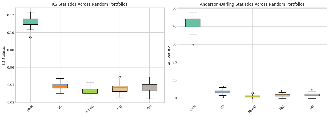
Distribution KS Mean KS Median KS Reject Rate AD Mean AD Median
NInvG 0.032845 0.032740 0.01 0.898434 0.797889
NIG 0.035985 0.037087 0.10 1.588689 1.574836
GH 0.037391 0.037722 0.19 1.863452 1.757622
VG 0.038414 0.038188 0.15 3.496930 3.348221
MVN 0.112396 0.112363 1.00 41.996915 41.885030
================================================================================
[19]:
# Visualize test statistics distribution
fig, axes = plt.subplots(1, 2, figsize=(14, 5))

# KS statistics boxplot
ax1 = axes[0]
ks_data = [portfolio_results[n]['ks_stats'] for n in fitted_dists.keys() if portfolio_results[n] is not None]
ks_labels = [n for n in fitted_dists.keys() if portfolio_results[n] is not None]
bp1 = ax1.boxplot(ks_data, labels=ks_labels, patch_artist=True)
for patch, color in zip(bp1['boxes'], colors[:len(ks_labels)]):
    patch.set_facecolor(color)
ax1.set_ylabel('KS Statistic')
ax1.set_title('KS Statistics Across Random Portfolios')
ax1.tick_params(axis='x', rotation=45)

# AD statistics boxplot
ax2 = axes[1]
ad_data = [portfolio_results[n]['ad_stats'] for n in fitted_dists.keys() if portfolio_results[n] is not None]
ad_labels = [n for n in fitted_dists.keys() if portfolio_results[n] is not None]
bp2 = ax2.boxplot(ad_data, labels=ad_labels, patch_artist=True)
for patch, color in zip(bp2['boxes'], colors[:len(ad_labels)]):
    patch.set_facecolor(color)
ax2.set_ylabel('AD Statistic')
ax2.set_title('Anderson-Darling Statistics Across Random Portfolios')
ax2.tick_params(axis='x', rotation=45)

plt.tight_layout()
plt.savefig('portfolio_test_boxplots.png', dpi=150, bbox_inches='tight')
plt.show()
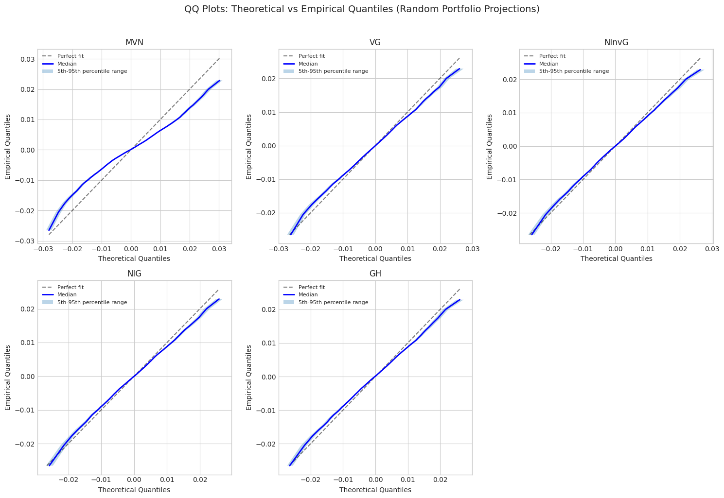
5. Quantile Range Plots
For each random portfolio, compare quantiles of simulated vs actual data.
[20]:
def compute_quantile_comparison(dist, returns_test, weights,
                                 quantiles=np.linspace(0.01, 0.99, 99),
                                 n_samples=10000, random_state=None):
    """
    Compute quantile comparison for multiple portfolios.

    Returns arrays of (empirical quantiles, theoretical quantiles) for each portfolio.
    """
    # Generate samples
    samples = dist.rvs(size=n_samples, random_state=random_state)

    n_portfolios = weights.shape[0]
    n_quantiles = len(quantiles)

    empirical_quantiles = np.zeros((n_portfolios, n_quantiles))
    theoretical_quantiles = np.zeros((n_portfolios, n_quantiles))

    for i in range(n_portfolios):
        w = weights[i]
        test_proj = returns_test @ w
        sample_proj = samples @ w

        empirical_quantiles[i] = np.quantile(test_proj, quantiles)
        theoretical_quantiles[i] = np.quantile(sample_proj, quantiles)

    return empirical_quantiles, theoretical_quantiles, quantiles
[21]:
# Compute quantile comparisons for select distributions
quantile_results = {}
quantiles = np.linspace(0.01, 0.99, 99)

for name, dist in fitted_dists.items():
    print(f"Computing quantiles for {name}...")
    try:
        emp_q, theo_q, q = compute_quantile_comparison(
            dist, returns_test, random_weights,
            quantiles=quantiles, n_samples=10000, random_state=42
        )
        quantile_results[name] = (emp_q, theo_q, q)
    except Exception as e:
        print(f"  Error: {e}")
Computing quantiles for MVN...
Computing quantiles for VG...
Computing quantiles for NInvG...
Computing quantiles for NIG...
Computing quantiles for GH...
[22]:
# Create QQ plot comparing all distributions
fig, axes = plt.subplots(2, 3, figsize=(15, 10))
axes = axes.flatten()

for idx, (name, (emp_q, theo_q, q)) in enumerate(quantile_results.items()):
    if idx >= len(axes):
        break
    ax = axes[idx]

    # Plot quantile range (5th-95th percentile across portfolios)
    emp_median = np.median(emp_q, axis=0)
    emp_lower = np.percentile(emp_q, 5, axis=0)
    emp_upper = np.percentile(emp_q, 95, axis=0)

    theo_median = np.median(theo_q, axis=0)
    theo_lower = np.percentile(theo_q, 5, axis=0)
    theo_upper = np.percentile(theo_q, 95, axis=0)

    # Plot diagonal
    min_val = min(emp_median.min(), theo_median.min())
    max_val = max(emp_median.max(), theo_median.max())
    ax.plot([min_val, max_val], [min_val, max_val], 'k--', alpha=0.5, label='Perfect fit')

    # Plot median QQ line
    ax.plot(theo_median, emp_median, 'b-', lw=2, label='Median')

    # Plot confidence band
    ax.fill_betweenx(emp_median, theo_lower, theo_upper, alpha=0.3,
                     label='5th-95th percentile range')

    ax.set_xlabel('Theoretical Quantiles')
    ax.set_ylabel('Empirical Quantiles')
    ax.set_title(f'{name}')
    ax.legend(loc='upper left', fontsize=8)

# Hide unused subplots
for idx in range(len(quantile_results), len(axes)):
    axes[idx].set_visible(False)

plt.suptitle('QQ Plots: Theoretical vs Empirical Quantiles (Random Portfolio Projections)',
             fontsize=14, y=1.02)
plt.tight_layout()
plt.savefig('qq_plots_comparison.png', dpi=150, bbox_inches='tight')
plt.show()
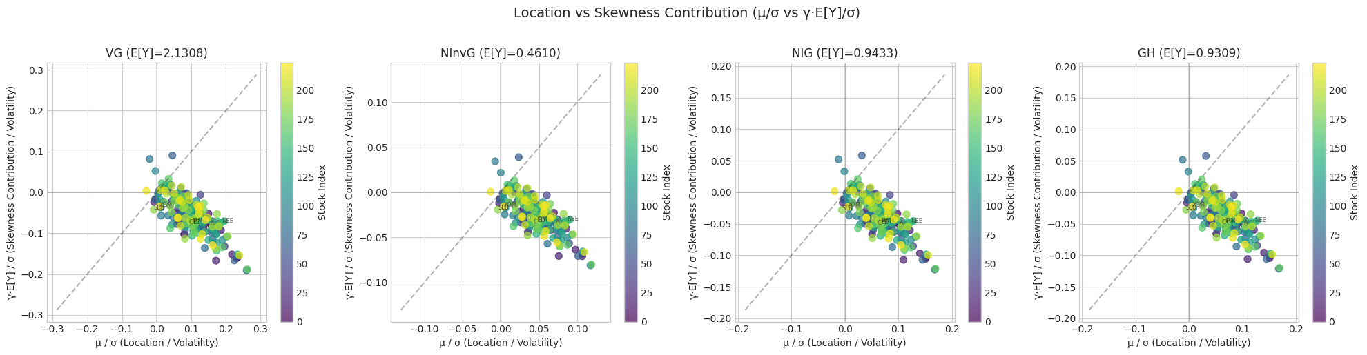
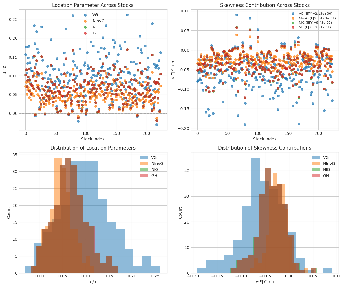
6. Parameter Analysis: Location (μ) vs Skewness (γ)
For normal mixture distributions, compare the location parameter μ and skewness parameter γ across stocks. We normalize by the volatility σ for comparison.
[27]:
# Extract parameters from fitted distributions
from normix.utils.bessel import log_kv

def compute_E_Y(name, params):
    """
    Compute E[Y] for the mixing distribution of each normal mixture type.

    - VG (Gamma):         E[Y] = α / β (shape / rate)
    - NInvG (InvGamma):   E[Y] = β / (α - 1) for α > 1 (rate / (shape - 1))
    - NIG (InvGaussian):  E[Y] = δ (delta)
    - GH (GIG):           E[Y] = √(b/a) * K_{p+1}(√(ab)) / K_p(√(ab))
    """
    if name == 'VG':
        alpha = params['shape']
        beta = params['rate']
        return alpha / beta
    elif name == 'NInvG':
        alpha = params['shape']
        beta = params['rate']
        if alpha > 1:
            return beta / (alpha - 1)
        else:
            return np.inf
    elif name == 'NIG':
        return params['delta']
    elif name == 'GH':
        p = params['p']
        a = params['a']
        b = params['b']
        sqrt_ab = np.sqrt(a * b)
        sqrt_b_over_a = np.sqrt(b / a) if a > 0 else np.inf
        log_kv_p = log_kv(p, sqrt_ab)
        log_kv_pp1 = log_kv(p + 1, sqrt_ab)
        E_Y = sqrt_b_over_a * np.exp(log_kv_pp1 - log_kv_p)
        return E_Y
    else:
        return 1.0  # Default for MVN or unknown

def extract_mixture_params(dist, name):
    """
    Extract μ, γ, σ (diagonal of Σ), and E[Y] from normal mixture distributions.

    Returns:
        mu: Location parameter
        gamma: Skewness parameter
        sigma_diag: Diagonal of covariance (volatilities)
        E_Y: Expected value of mixing variable
        full_params: All classical parameters
        mix_params: Mixing distribution parameters
    """
    if name == 'MVN':
        params = dist.classical_params
        mu = params.mu
        sigma_diag = np.sqrt(np.diag(params.sigma))
        gamma = np.zeros_like(mu)  # No skewness parameter for MVN
        E_Y = 1.0  # MVN is not a mixture
        return mu, gamma, sigma_diag, E_Y, None, None
    else:
        params = dist.classical_params
        mu = params.mu
        gamma = params.gamma
        sigma_diag = np.sqrt(np.diag(params.sigma))

        # Get mixing distribution parameters
        if name == 'VG':
            mix_params = {'shape': params.shape, 'rate': params.rate}
        elif name == 'NInvG':
            mix_params = {'shape': params.shape, 'rate': params.rate}
        elif name == 'NIG':
            mix_params = {'delta': params.delta, 'eta': params.eta}
        elif name == 'GH':
            mix_params = {'p': params.p, 'a': params.a, 'b': params.b}
        else:
            mix_params = None

        # Compute E[Y]
        E_Y = compute_E_Y(name, params)

        return mu, gamma, sigma_diag, E_Y, params, mix_params

# Extract parameters for all mixture distributions
param_data = {}
for name, dist in fitted_dists.items():
    try:
        mu, gamma, sigma, E_Y, full_params, mix_params = extract_mixture_params(dist, name)
        param_data[name] = {
            'mu': mu,
            'gamma': gamma,
            'sigma': sigma,
            'E_Y': E_Y,
            'mu_over_sigma': mu / sigma,
            'gamma_over_sigma': gamma / sigma,
            'gamma_E_Y_over_sigma': gamma * E_Y / sigma,  # The comparable quantity
            'full_params': full_params,
            'mix_params': mix_params
        }
        print(f"{name}: μ range [{mu.min():.6f}, {mu.max():.6f}], γ range [{gamma.min():.6f}, {gamma.max():.6f}], E[Y] = {E_Y:.6f}")
        print(f"       γ*E[Y] range [{(gamma*E_Y).min():.6f}, {(gamma*E_Y).max():.6f}]")
    except Exception as e:
        print(f"Error extracting params for {name}: {e}")
MVN: μ range [-0.000885, 0.002879], γ range [0.000000, 0.000000], E[Y] = 1.000000
       γ*E[Y] range [0.000000, 0.000000]
VG: μ range [-0.000381, 0.004421], γ range [-0.000963, 0.000496], E[Y] = 2.130790
       γ*E[Y] range [-0.002052, 0.001057]
NInvG: μ range [-0.000356, 0.004371], γ range [-0.004009, 0.002058], E[Y] = 0.460976
       γ*E[Y] range [-0.001848, 0.000949]
NIG: μ range [-0.000369, 0.004393], γ range [-0.002111, 0.001086], E[Y] = 0.943274
       γ*E[Y] range [-0.001992, 0.001025]
GH: μ range [-0.000369, 0.004396], γ range [-0.002117, 0.001089], E[Y] = 0.930902
       γ*E[Y] range [-0.001971, 0.001014]
[28]:
# Create scatter plots comparing μ/σ vs γ*E[Y]/σ for each stock
# Note: For normal mixture X = μ + γY + √Y * Z, the contribution of γ to E[X] is γ*E[Y]
# So comparing μ/σ to γ*E[Y]/σ gives a better sense of relative contributions
mixture_dists = [n for n in ['VG', 'NInvG', 'NIG', 'GH'] if n in param_data]

if mixture_dists:
    n_plots = len(mixture_dists)
    fig, axes = plt.subplots(1, n_plots, figsize=(5*n_plots, 5))
    if n_plots == 1:
        axes = [axes]

    for idx, name in enumerate(mixture_dists):
        ax = axes[idx]
        data = param_data[name]

        mu_norm = data['mu_over_sigma']
        gamma_E_Y_norm = data['gamma_E_Y_over_sigma']  # γ*E[Y]/σ instead of γ/σ

        # Scatter plot
        scatter = ax.scatter(mu_norm, gamma_E_Y_norm, c=range(len(mu_norm)),
                            cmap='viridis', s=50, alpha=0.7)

        # Add diagonal line
        lim = max(abs(mu_norm).max(), abs(gamma_E_Y_norm).max()) * 1.1
        if np.isfinite(lim) and lim > 0:
            ax.plot([-lim, lim], [-lim, lim], 'k--', alpha=0.3, label='μ = γE[Y]')
        ax.axhline(0, color='gray', linestyle='-', alpha=0.3)
        ax.axvline(0, color='gray', linestyle='-', alpha=0.3)

        # Labels
        ax.set_xlabel('μ / σ (Location / Volatility)')
        ax.set_ylabel('γ·E[Y] / σ (Skewness Contribution / Volatility)')
        ax.set_title(f'{name} (E[Y]={data["E_Y"]:.4f})')

        # Add colorbar to show stock index
        plt.colorbar(scatter, ax=ax, label='Stock Index')

        # Add labels for a few interesting points
        n_labels = min(len(selected_tickers), 6)  # Label up to 6 stocks
        step = max(1, len(selected_tickers) // n_labels)
        for i, ticker in enumerate(selected_tickers):
            if i % step == 0:
                ax.annotate(ticker, (mu_norm[i], gamma_E_Y_norm[i]), fontsize=6, alpha=0.7)

    plt.suptitle('Location vs Skewness Contribution (μ/σ vs γ·E[Y]/σ)', fontsize=14, y=1.02)
    plt.tight_layout()
    plt.savefig('mu_vs_gamma_E_Y_scatter.png', dpi=150, bbox_inches='tight')
    plt.show()
[29]:
# Create combined comparison plot using γ*E[Y]/σ for fair comparison
if len(mixture_dists) >= 2:
    fig, axes = plt.subplots(2, 2, figsize=(12, 10))

    # Plot 1: μ/σ comparison across distributions
    ax1 = axes[0, 0]
    for name in mixture_dists:
        data = param_data[name]
        ax1.scatter(range(len(data['mu_over_sigma'])), data['mu_over_sigma'],
                   label=name, alpha=0.7, s=30)
    ax1.set_xlabel('Stock Index')
    ax1.set_ylabel('μ / σ')
    ax1.set_title('Location Parameter Across Stocks')
    ax1.legend()
    ax1.axhline(0, color='gray', linestyle='--', alpha=0.5)

    # Plot 2: γ*E[Y]/σ comparison across distributions (scaled skewness contribution)
    ax2 = axes[0, 1]
    for name in mixture_dists:
        data = param_data[name]
        ax2.scatter(range(len(data['gamma_E_Y_over_sigma'])), data['gamma_E_Y_over_sigma'],
                   label=f"{name} (E[Y]={data['E_Y']:.2e})", alpha=0.7, s=30)
    ax2.set_xlabel('Stock Index')
    ax2.set_ylabel('γ·E[Y] / σ')
    ax2.set_title('Skewness Contribution Across Stocks')
    ax2.legend(fontsize=8)
    ax2.axhline(0, color='gray', linestyle='--', alpha=0.5)

    # Plot 3: μ/σ histograms
    ax3 = axes[1, 0]
    for name in mixture_dists:
        data = param_data[name]
        ax3.hist(data['mu_over_sigma'], bins=15, alpha=0.5, label=name)
    ax3.set_xlabel('μ / σ')
    ax3.set_ylabel('Count')
    ax3.set_title('Distribution of Location Parameters')
    ax3.legend()

    # Plot 4: γ*E[Y]/σ histograms (scaled skewness contribution)
    ax4 = axes[1, 1]
    for name in mixture_dists:
        data = param_data[name]
        ax4.hist(data['gamma_E_Y_over_sigma'], bins=15, alpha=0.5, label=name)
    ax4.set_xlabel('γ·E[Y] / σ')
    ax4.set_ylabel('Count')
    ax4.set_title('Distribution of Skewness Contributions')
    ax4.legend()

    plt.tight_layout()
    plt.savefig('parameter_comparison.png', dpi=150, bbox_inches='tight')
    plt.show()
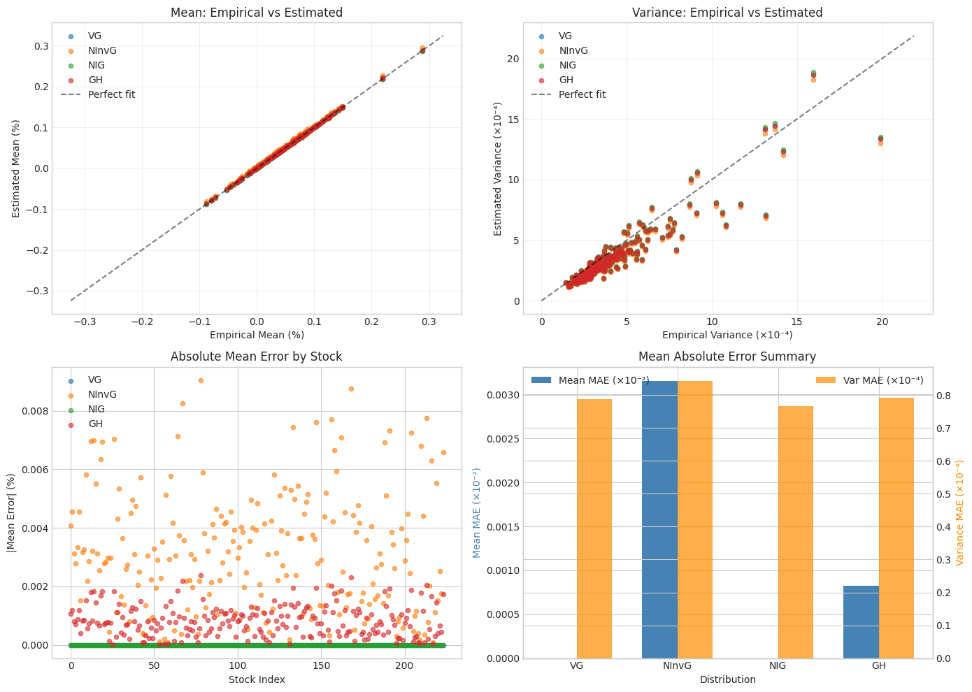
[30]:
# Compare Mean, Variance, and Skewness from Estimated Distributions
# For normal variance-mean mixture X = μ + γY + √Y·ε where ε ~ N(0, Σ):
# - E[X] = μ + γE[Y]
# - Var[X]_i = E[Y]·Σ_ii + Var[Y]·γ_i²

def compute_Var_Y(name, params):
    """
    Compute Var[Y] for the mixing distribution.

    - VG (Gamma):         Var[Y] = α / β² (shape / rate²)
    - NInvG (InvGamma):   Var[Y] = β² / ((α-1)²(α-2)) for α > 2
    - NIG (InvGaussian):  Var[Y] = δ³ / η (delta³ / eta)
    - GH (GIG):           Var[Y] = E[Y²] - E[Y]² computed via Bessel ratios
    """
    if name == 'VG':
        alpha = params['shape']
        beta = params['rate']
        return alpha / (beta ** 2)
    elif name == 'NInvG':
        alpha = params['shape']
        beta = params['rate']
        if alpha > 2:
            return (beta ** 2) / ((alpha - 1) ** 2 * (alpha - 2))
        else:
            return np.inf
    elif name == 'NIG':
        delta = params['delta']
        eta = params['eta']
        return (delta ** 3) / eta
    elif name == 'GH':
        p = params['p']
        a = params['a']
        b = params['b']
        sqrt_ab = np.sqrt(a * b)
        sqrt_b_over_a = np.sqrt(b / a) if a > 0 else np.inf
        log_kv_p = log_kv(p, sqrt_ab)
        log_kv_pp1 = log_kv(p + 1, sqrt_ab)
        log_kv_pp2 = log_kv(p + 2, sqrt_ab)
        E_Y = sqrt_b_over_a * np.exp(log_kv_pp1 - log_kv_p)
        E_Y2 = (b / a) * np.exp(log_kv_pp2 - log_kv_p)
        return E_Y2 - E_Y ** 2
    else:
        return 0.0

print("="*80)
print("MOMENT COMPARISON FROM ESTIMATED DISTRIBUTIONS")
print("="*80)

# Compare empirical moments with distribution moments
empirical_mean = returns_train.mean(axis=0)
empirical_var = returns_train.var(axis=0)
empirical_skew = stats.skew(returns_train, axis=0)

moment_comparison = {}

for name in mixture_dists:
    data = param_data[name]
    mu = data['mu']
    gamma = data['gamma']
    sigma_diag_sq = data['sigma'] ** 2  # Variance (diagonal of Σ)
    E_Y = data['E_Y']
    Var_Y = compute_Var_Y(name, data['full_params'])

    # Compute distribution mean: E[X] = μ + γE[Y]
    dist_mean = mu + gamma * E_Y

    # Compute distribution variance: Var[X]_i = E[Y]·Σ_ii + Var[Y]·γ_i²
    dist_var = E_Y * sigma_diag_sq + Var_Y * (gamma ** 2)

    moment_comparison[name] = {
        'E_Y': E_Y,
        'Var_Y': Var_Y,
        'dist_mean': dist_mean,
        'dist_var': dist_var,
        'dist_std': np.sqrt(dist_var),
        'mean_error': np.mean(np.abs(dist_mean - empirical_mean)),
        'var_error': np.mean(np.abs(dist_var - empirical_var))
    }

    print(f"\n{name}:")
    print(f"  E[Y] = {E_Y:.6e}, Var[Y] = {Var_Y:.6e}")
    print(f"  Mean: Dist avg = {dist_mean.mean():.6e}, Empirical avg = {empirical_mean.mean():.6e}")
    print(f"         MAE = {moment_comparison[name]['mean_error']:.6e}")
    print(f"  Var:  Dist avg = {dist_var.mean():.6e}, Empirical avg = {empirical_var.mean():.6e}")
    print(f"         MAE = {moment_comparison[name]['var_error']:.6e}")

# Create comparison visualization
fig, axes = plt.subplots(2, 2, figsize=(14, 10))

# Plot 1: Mean comparison (scatter: empirical vs estimated)
ax1 = axes[0, 0]
for name in mixture_dists:
    mc = moment_comparison[name]
    ax1.scatter(empirical_mean * 100, mc['dist_mean'] * 100, label=name, alpha=0.6, s=20)
# Add diagonal line
lim = max(abs(empirical_mean).max(), max(abs(mc['dist_mean']).max() for mc in moment_comparison.values())) * 100 * 1.1
ax1.plot([-lim, lim], [-lim, lim], 'k--', alpha=0.5, label='Perfect fit')
ax1.set_xlabel('Empirical Mean (%)')
ax1.set_ylabel('Estimated Mean (%)')
ax1.set_title('Mean: Empirical vs Estimated')
ax1.legend()
ax1.grid(True, alpha=0.3)

# Plot 2: Variance comparison (scatter: empirical vs estimated)
ax2 = axes[0, 1]
for name in mixture_dists:
    mc = moment_comparison[name]
    ax2.scatter(empirical_var * 10000, mc['dist_var'] * 10000, label=name, alpha=0.6, s=20)
lim = max(empirical_var.max(), max(mc['dist_var'].max() for mc in moment_comparison.values() if np.isfinite(mc['dist_var']).all())) * 10000 * 1.1
ax2.plot([0, lim], [0, lim], 'k--', alpha=0.5, label='Perfect fit')
ax2.set_xlabel('Empirical Variance (×10⁻⁴)')
ax2.set_ylabel('Estimated Variance (×10⁻⁴)')
ax2.set_title('Variance: Empirical vs Estimated')
ax2.legend()
ax2.grid(True, alpha=0.3)

# Plot 3: Mean error by stock
ax3 = axes[1, 0]
for name in mixture_dists:
    mc = moment_comparison[name]
    mean_errors = np.abs(mc['dist_mean'] - empirical_mean) * 100
    ax3.scatter(range(len(mean_errors)), mean_errors, label=name, alpha=0.6, s=20)
ax3.set_xlabel('Stock Index')
ax3.set_ylabel('|Mean Error| (%)')
ax3.set_title('Absolute Mean Error by Stock')
ax3.legend()

# Plot 4: Summary statistics
ax4 = axes[1, 1]
names = list(moment_comparison.keys())
mean_maes = [moment_comparison[n]['mean_error'] * 100 for n in names]
var_maes = [moment_comparison[n]['var_error'] * 10000 for n in names]

x = np.arange(len(names))
width = 0.35
bars1 = ax4.bar(x - width/2, mean_maes, width, label='Mean MAE (×10⁻²)', color='steelblue')
ax4_twin = ax4.twinx()
bars2 = ax4_twin.bar(x + width/2, var_maes, width, label='Var MAE (×10⁻⁴)', color='darkorange', alpha=0.7)

ax4.set_xlabel('Distribution')
ax4.set_ylabel('Mean MAE (×10⁻²)', color='steelblue')
ax4_twin.set_ylabel('Variance MAE (×10⁻⁴)', color='darkorange')
ax4.set_xticks(x)
ax4.set_xticklabels(names)
ax4.set_title('Mean Absolute Error Summary')
ax4.legend(loc='upper left')
ax4_twin.legend(loc='upper right')

plt.tight_layout()
plt.savefig('moment_comparison.png', dpi=150, bbox_inches='tight')
plt.show()

# Print summary table
print("\n" + "="*80)
print("SUMMARY TABLE: Distribution Moment Comparison")
print("="*80)
summary_df = pd.DataFrame({
    'Distribution': names,
    'E[Y]': [moment_comparison[n]['E_Y'] for n in names],
    'Var[Y]': [moment_comparison[n]['Var_Y'] for n in names],
    'Mean MAE': [moment_comparison[n]['mean_error'] for n in names],
    'Var MAE': [moment_comparison[n]['var_error'] for n in names]
})
print(summary_df.to_string(index=False))
================================================================================
MOMENT COMPARISON FROM ESTIMATED DISTRIBUTIONS
================================================================================

VG:
  E[Y] = 2.130790e+00, Var[Y] = 2.229780e+00
  Mean: Dist avg = 5.226405e-04, Empirical avg = 5.226405e-04
         MAE = 2.464937e-17
  Var:  Dist avg = 3.526543e-04, Empirical avg = 4.178537e-04
         MAE = 7.873155e-05

NInvG:
  E[Y] = 4.609764e-01, Var[Y] = 2.382077e-01
  Mean: Dist avg = 5.522672e-04, Empirical avg = 5.226405e-04
         MAE = 3.157227e-05
  Var:  Dist avg = 3.439041e-04, Empirical avg = 4.178537e-04
         MAE = 8.438055e-05

NIG:
  E[Y] = 9.432736e-01, Var[Y] = 5.249672e-01
  Mean: Dist avg = 5.226405e-04, Empirical avg = 5.226405e-04
         MAE = 1.786790e-17
  Var:  Dist avg = 3.567892e-04, Empirical avg = 4.178537e-04
         MAE = 7.660339e-05

GH:
  E[Y] = 9.309021e-01, Var[Y] = 4.867629e-01
  Mean: Dist avg = 5.303291e-04, Empirical avg = 5.226405e-04
         MAE = 8.222104e-06
  Var:  Dist avg = 3.521624e-04, Empirical avg = 4.178537e-04
         MAE = 7.925527e-05
================================================================================
SUMMARY TABLE: Distribution Moment Comparison
================================================================================
Distribution     E[Y]   Var[Y]     Mean MAE  Var MAE
          VG 2.130790 2.229780 2.464937e-17 0.000079
       NInvG 0.460976 0.238208 3.157227e-05 0.000084
         NIG 0.943274 0.524967 1.786790e-17 0.000077
          GH 0.930902 0.486763 8.222104e-06 0.000079
[31]:
# Create a detailed parameter table for one distribution (e.g., GH)
best_dist = 'GH' if 'GH' in param_data else list(param_data.keys())[-1]

if best_dist in param_data:
    data = param_data[best_dist]

    param_table = pd.DataFrame({
        'Ticker': selected_tickers,
        'μ': data['mu'],
        'γ': data['gamma'],
        'γ·E[Y]': data['gamma'] * data['E_Y'],  # Skewness contribution
        'σ': data['sigma'],
        'μ/σ': data['mu_over_sigma'],
        'γ/σ': data['gamma_over_sigma'],
        'γ·E[Y]/σ': data['gamma_E_Y_over_sigma']  # Comparable skewness measure
    })

    # Sort by γ*E[Y]/σ to see which stocks have most skewness contribution
    param_table_sorted = param_table.sort_values('γ·E[Y]/σ')

    print(f"\n{best_dist} Parameters by Stock (sorted by skewness contribution γ·E[Y]/σ):")
    print(f"Note: E[Y] = {data['E_Y']:.6e}")
    print("="*100)
    print(param_table_sorted.to_string(index=False))
    print("="*100)

    # Print mixing distribution parameters
    if data['mix_params']:
        print(f"\n{best_dist} Mixing Distribution Parameters:")
        for k, v in data['mix_params'].items():
            if isinstance(v, float):
                print(f"  {k}: {v:.6e}")
            else:
                print(f"  {k}: {v}")
GH Parameters by Stock (sorted by skewness contribution γ·E[Y]/σ):
Note: E[Y] = 9.309021e-01
====================================================================================================
Ticker         μ         γ    γ·E[Y]        σ       μ/σ       γ/σ  γ·E[Y]/σ
  EQIX  0.002732 -0.002117 -0.001971 0.016250  0.168124 -0.130298 -0.121294
   PLD  0.002697 -0.002047 -0.001905 0.015900  0.169643 -0.128726 -0.119831
   AVB  0.001572 -0.001632 -0.001519 0.014332  0.109678 -0.113883 -0.106014
   DLR  0.002471 -0.001936 -0.001802 0.017023  0.145175 -0.113722 -0.105864
   BAX  0.002180 -0.001620 -0.001508 0.014438  0.150969 -0.112205 -0.104452
   AMT  0.002267 -0.001627 -0.001515 0.014909  0.152069 -0.109153 -0.101611
     V  0.002322 -0.001581 -0.001472 0.014910  0.155760 -0.106027 -0.098701
   MCO  0.002518 -0.001727 -0.001608 0.016513  0.152459 -0.104580 -0.097354
   ARE  0.002036 -0.001493 -0.001389 0.014504  0.140361 -0.102904 -0.095794
     O  0.001797 -0.001570 -0.001461 0.016166  0.111162 -0.097088 -0.090379
   STZ  0.001997 -0.001702 -0.001585 0.018145  0.110075 -0.093823 -0.087340
   PEP  0.001399 -0.001050 -0.000978 0.011309  0.123745 -0.092881 -0.086463
   EQR  0.001334 -0.001387 -0.001292 0.015030  0.088731 -0.092311 -0.085933
   CCI  0.001874 -0.001332 -0.001240 0.014684  0.127649 -0.090706 -0.084438
   ZBH  0.001811 -0.001532 -0.001426 0.017278  0.104799 -0.088642 -0.082517
    KO  0.001222 -0.000984 -0.000916 0.011452  0.106712 -0.085904 -0.079968
   LMT  0.001580 -0.001186 -0.001104 0.013962  0.113161 -0.084938 -0.079069
  MDLZ  0.001393 -0.001155 -0.001075 0.014290  0.097484 -0.080795 -0.075212
   ICE  0.001774 -0.001155 -0.001075 0.014357  0.123588 -0.080427 -0.074869
   DHI  0.002192 -0.001652 -0.001538 0.020822  0.105276 -0.079321 -0.073840
  WELL  0.001554 -0.001477 -0.001375 0.018990  0.081835 -0.077775 -0.072401
   SPG  0.001088 -0.001631 -0.001518 0.021141  0.051467 -0.077130 -0.071801
    MA  0.002202 -0.001246 -0.001160 0.016652  0.132255 -0.074842 -0.069671
  SPGI  0.002147 -0.001185 -0.001103 0.016006  0.134159 -0.074051 -0.068934
    MO  0.001023 -0.001128 -0.001050 0.015396  0.066440 -0.073286 -0.068222
   MCD  0.001392 -0.000879 -0.000818 0.012290  0.113236 -0.071493 -0.066553
   AIG  0.000979 -0.001355 -0.001261 0.019193  0.051021 -0.070595 -0.065717
   FIS  0.001635 -0.001023 -0.000952 0.014644  0.111645 -0.069834 -0.065009
   MMM  0.001162 -0.001032 -0.000960 0.014796  0.078518 -0.069717 -0.064899
  VRTX  0.002219 -0.001820 -0.001694 0.026254  0.084504 -0.069306 -0.064518
    ES  0.001361 -0.000889 -0.000828 0.013156  0.103473 -0.067569 -0.062900
   PSA  0.001003 -0.000989 -0.000920 0.014670  0.068347 -0.067403 -0.062746
   NOC  0.001381 -0.001019 -0.000949 0.015285  0.090336 -0.066674 -0.062067
   BDX  0.001380 -0.000995 -0.000926 0.014946  0.092338 -0.066557 -0.061958
    HD  0.001503 -0.000921 -0.000858 0.014127  0.106411 -0.065214 -0.060708
    PM  0.001116 -0.001026 -0.000955 0.015773  0.070738 -0.065070 -0.060574
    GD  0.001016 -0.000955 -0.000889 0.014742  0.068937 -0.064767 -0.060291
  AMZN  0.002434 -0.001279 -0.001191 0.020011  0.121648 -0.063916 -0.059500
   CVS  0.000986 -0.001187 -0.001105 0.018650  0.052868 -0.063645 -0.059247
   MET  0.001381 -0.001259 -0.001172 0.019795  0.069788 -0.063618 -0.059223
   LEN  0.001626 -0.001352 -0.001259 0.022065  0.073712 -0.061272 -0.057038
   OXY  0.000671 -0.001652 -0.001538 0.027419  0.024487 -0.060244 -0.056081
   EXR  0.001270 -0.000981 -0.000913 0.016287  0.078008 -0.060225 -0.056063
   MKC  0.001488 -0.000857 -0.000797 0.014335  0.103816 -0.059761 -0.055632
   MCK  0.001131 -0.001218 -0.001134 0.020780  0.054418 -0.058632 -0.054580
  ISRG  0.002259 -0.001114 -0.001037 0.019096  0.118292 -0.058347 -0.054315
   AEP  0.001120 -0.000738 -0.000687 0.012701  0.088154 -0.058070 -0.054058
   TMO  0.001859 -0.000914 -0.000851 0.015750  0.118044 -0.058033 -0.054023
   SYK  0.001642 -0.000897 -0.000835 0.015508  0.105871 -0.057843 -0.053846
   BSX  0.001485 -0.001038 -0.000966 0.018023  0.082368 -0.057570 -0.053592
   UAL  0.001311 -0.001666 -0.001551 0.029172  0.044947 -0.057100 -0.053154
    CL  0.000951 -0.000709 -0.000660 0.012438  0.076432 -0.056963 -0.053027
   RTX  0.001089 -0.000934 -0.000870 0.016431  0.066274 -0.056848 -0.052920
     A  0.001762 -0.000945 -0.000879 0.017206  0.102394 -0.054908 -0.051114
   PPG  0.001177 -0.000904 -0.000842 0.016506  0.071295 -0.054778 -0.050993
  AAPL  0.002220 -0.001045 -0.000973 0.019162  0.115872 -0.054547 -0.050778
  NVDA  0.003874 -0.001784 -0.001661 0.032714  0.118435 -0.054539 -0.050771
     C  0.001262 -0.001137 -0.001058 0.020852  0.060513 -0.054521 -0.050754
   DAL  0.001126 -0.001320 -0.001228 0.024302  0.046323 -0.054302 -0.050550
   KHC  0.000507 -0.000966 -0.000899 0.017869  0.028381 -0.054043 -0.050309
 GOOGL  0.001484 -0.000895 -0.000834 0.016625  0.089292 -0.053864 -0.050142
   ETR  0.001158 -0.000753 -0.000701 0.013986  0.082796 -0.053838 -0.050118
   PRU  0.001114 -0.001091 -0.001015 0.020330  0.054810 -0.053656 -0.049949
   CAH  0.000774 -0.001100 -0.001024 0.020535  0.037678 -0.053557 -0.049856
   KMB  0.000888 -0.000726 -0.000675 0.013581  0.065409 -0.053424 -0.049733
  ADBE  0.002312 -0.001047 -0.000975 0.019677  0.117509 -0.053227 -0.049549
   IBM  0.000867 -0.000820 -0.000763 0.015441  0.056130 -0.053089 -0.049421
    ED  0.000877 -0.000685 -0.000637 0.012897  0.067963 -0.053080 -0.049412
   OKE  0.001942 -0.001348 -0.001255 0.025807  0.075261 -0.052251 -0.048640
    MU  0.002923 -0.001735 -0.001615 0.033660  0.086840 -0.051535 -0.047974
   IRM  0.001178 -0.000911 -0.000848 0.017674  0.066628 -0.051521 -0.047961
     D  0.000894 -0.000681 -0.000634 0.013227  0.067620 -0.051495 -0.047936
   NEE  0.001577 -0.000651 -0.000606 0.012842  0.122822 -0.050710 -0.047206
   ACN  0.001475 -0.000768 -0.000715 0.015193  0.097062 -0.050540 -0.047048
  MSFT  0.001930 -0.000826 -0.000769 0.016629  0.116051 -0.049702 -0.046268
    GM  0.001240 -0.001045 -0.000973 0.021068  0.058872 -0.049621 -0.046192
  BIIB  0.001039 -0.001234 -0.001149 0.025054  0.041455 -0.049258 -0.045855
    DD  0.000901 -0.000962 -0.000896 0.019746  0.045623 -0.048719 -0.045352
  MSCI  0.002315 -0.000876 -0.000816 0.018103  0.127866 -0.048406 -0.045061
   AWK  0.001448 -0.000664 -0.000619 0.013753  0.105292 -0.048313 -0.044975
   NOW  0.002555 -0.001204 -0.001121 0.024948  0.102428 -0.048274 -0.044938
  GOOG  0.001409 -0.000803 -0.000747 0.016646  0.084667 -0.048223 -0.044891
   LOW  0.001496 -0.000891 -0.000829 0.018486  0.080918 -0.048176 -0.044847
  CSCO  0.001296 -0.000821 -0.000764 0.017133  0.075643 -0.047904 -0.044594
   TRV  0.000881 -0.000670 -0.000623 0.013997  0.062944 -0.047843 -0.044537
   HLT  0.001555 -0.000888 -0.000826 0.018648  0.083406 -0.047596 -0.044307
   LIN  0.001460 -0.000725 -0.000675 0.015371  0.094953 -0.047196 -0.043935
   XEL  0.001166 -0.000589 -0.000548 0.012729  0.091638 -0.046238 -0.043043
  INTC  0.001254 -0.000923 -0.000859 0.019972  0.062772 -0.046204 -0.043012
  COST  0.001391 -0.000656 -0.000611 0.014393  0.096610 -0.045602 -0.042451
   SYY  0.001284 -0.000786 -0.000731 0.017464  0.073502 -0.044992 -0.041884
  AMGN  0.001091 -0.000740 -0.000689 0.016495  0.066125 -0.044881 -0.041780
   WMB  0.001168 -0.001282 -0.001194 0.029333  0.039835 -0.043714 -0.040694
     T  0.000755 -0.000598 -0.000557 0.013768  0.054870 -0.043463 -0.040460
  BKNG  0.001199 -0.000845 -0.000787 0.019573  0.061271 -0.043192 -0.040208
     F  0.000618 -0.000836 -0.000778 0.019486  0.031705 -0.042891 -0.039927
  TTWO  0.002347 -0.001046 -0.000974 0.024457  0.095949 -0.042768 -0.039813
   MPC  0.001074 -0.001189 -0.001107 0.027802  0.038617 -0.042755 -0.039800
  META  0.001533 -0.000841 -0.000783 0.019729  0.077708 -0.042632 -0.039686
   VLO  0.000958 -0.001024 -0.000953 0.024033  0.039858 -0.042595 -0.039652
   HSY  0.001065 -0.000569 -0.000530 0.013364  0.079708 -0.042580 -0.039638
   PEG  0.000987 -0.000586 -0.000545 0.013757  0.071755 -0.042562 -0.039621
  NXPI  0.001440 -0.000978 -0.000910 0.023230  0.061997 -0.042098 -0.039189
    CB  0.000846 -0.000582 -0.000542 0.014301  0.059168 -0.040698 -0.037886
   AXP  0.001123 -0.000687 -0.000640 0.016892  0.066495 -0.040689 -0.037878
   ABT  0.001372 -0.000636 -0.000592 0.015634  0.087727 -0.040683 -0.037872
   APD  0.001260 -0.000588 -0.000548 0.014666  0.085902 -0.040106 -0.037334
  GILD  0.000398 -0.000725 -0.000675 0.018148  0.021909 -0.039933 -0.037174
    GE  0.000195 -0.000973 -0.000906 0.024830  0.007842 -0.039187 -0.036479
   DTE  0.000932 -0.000512 -0.000476 0.013091  0.071166 -0.039100 -0.036398
   ALL  0.000980 -0.000509 -0.000474 0.013247  0.073999 -0.038417 -0.035763
    DG  0.001553 -0.000700 -0.000651 0.018308  0.084844 -0.038219 -0.035578
   GIS  0.000686 -0.000573 -0.000533 0.015073  0.045492 -0.037992 -0.035367
   SHW  0.001385 -0.000602 -0.000560 0.015891  0.087141 -0.037857 -0.035241
  ABBV  0.001338 -0.000710 -0.000661 0.018755  0.071316 -0.037839 -0.035224
   MDT  0.000914 -0.000543 -0.000506 0.014441  0.063265 -0.037628 -0.035028
   AES  0.001586 -0.000759 -0.000706 0.020194  0.078516 -0.037579 -0.034982
  DLTR  0.001010 -0.000815 -0.000758 0.021700  0.046566 -0.037540 -0.034946
  SNPS  0.001948 -0.000631 -0.000588 0.016921  0.115115 -0.037317 -0.034738
   CAG  0.000884 -0.000721 -0.000671 0.019531  0.045272 -0.036902 -0.034352
   WEC  0.001031 -0.000471 -0.000438 0.012958  0.079573 -0.036310 -0.033801
   AMD  0.004396 -0.001610 -0.001499 0.044745  0.098241 -0.035980 -0.033494
   COF  0.000979 -0.000747 -0.000695 0.021300  0.045962 -0.035053 -0.032631
   BLK  0.001234 -0.000599 -0.000558 0.017174  0.071823 -0.034874 -0.032464
    PG  0.000942 -0.000398 -0.000371 0.011539  0.081673 -0.034528 -0.032142
   CME  0.001161 -0.000519 -0.000483 0.015035  0.077201 -0.034524 -0.032138
   BMY  0.000624 -0.000631 -0.000587 0.018327  0.034066 -0.034411 -0.032033
   EXC  0.000954 -0.000502 -0.000468 0.014647  0.065155 -0.034298 -0.031928
  REGN  0.000681 -0.000827 -0.000770 0.024656  0.027616 -0.033546 -0.031228
    EA  0.001245 -0.000711 -0.000662 0.021763  0.057206 -0.032662 -0.030406
   JNJ  0.000809 -0.000391 -0.000364 0.012143  0.066608 -0.032202 -0.029977
   ECL  0.000942 -0.000447 -0.000416 0.013949  0.067501 -0.032068 -0.029853
   HON  0.001099 -0.000445 -0.000414 0.013966  0.078709 -0.031865 -0.029663
   TXN  0.001454 -0.000558 -0.000519 0.018001  0.080791 -0.031000 -0.028858
  SBUX  0.000931 -0.000475 -0.000442 0.015324  0.060786 -0.030995 -0.028853
   LLY  0.001100 -0.000502 -0.000467 0.016426  0.066949 -0.030560 -0.028448
   ITW  0.001159 -0.000471 -0.000438 0.015581  0.074415 -0.030232 -0.028143
   SLB -0.000129 -0.000705 -0.000657 0.023589 -0.005484 -0.029906 -0.027840
   RSG  0.000989 -0.000330 -0.000308 0.011088  0.089237 -0.029800 -0.027741
    BA  0.000981 -0.000667 -0.000621 0.023712  0.041379 -0.028147 -0.026202
  AVGO  0.001555 -0.000621 -0.000578 0.022465  0.069237 -0.027639 -0.025729
  FTNT  0.001788 -0.000654 -0.000609 0.023825  0.075025 -0.027468 -0.025570
   SRE  0.000713 -0.000390 -0.000363 0.014448  0.049322 -0.026992 -0.025127
   HAL  0.000227 -0.000746 -0.000695 0.027851  0.008163 -0.026793 -0.024941
   MAR  0.001041 -0.000550 -0.000512 0.020690  0.050294 -0.026588 -0.024750
  AMAT  0.001864 -0.000654 -0.000609 0.025178  0.074037 -0.025964 -0.024170
  ORCL  0.000848 -0.000414 -0.000385 0.016009  0.052964 -0.025857 -0.024070
   NSC  0.001295 -0.000469 -0.000436 0.018322  0.070670 -0.025574 -0.023807
    SO  0.000697 -0.000320 -0.000298 0.013029  0.053529 -0.024579 -0.022881
   XOM  0.000091 -0.000400 -0.000372 0.016267  0.005606 -0.024571 -0.022873
  LRCX  0.002068 -0.000617 -0.000575 0.025148  0.082245 -0.024550 -0.022854
   WMT  0.001132 -0.000351 -0.000327 0.014340  0.078938 -0.024474 -0.022783
   CRM  0.001288 -0.000520 -0.000484 0.021490  0.059921 -0.024218 -0.022544
   FDX  0.000941 -0.000496 -0.000461 0.020536  0.045798 -0.024134 -0.022466
   SJM  0.000427 -0.000387 -0.000361 0.016271  0.026216 -0.023814 -0.022168
   DUK  0.000647 -0.000284 -0.000265 0.012360  0.052350 -0.023013 -0.021423
   CAT  0.001350 -0.000462 -0.000430 0.020097  0.067196 -0.023003 -0.021413
    WM  0.000952 -0.000260 -0.000242 0.011398  0.083487 -0.022770 -0.021196
  NFLX  0.001739 -0.000649 -0.000605 0.028627  0.060758 -0.022687 -0.021120
    BK  0.000437 -0.000384 -0.000358 0.017224  0.025351 -0.022303 -0.020762
   PFE  0.000569 -0.000295 -0.000275 0.013732  0.041426 -0.021483 -0.019998
  TSLA  0.002960 -0.000820 -0.000764 0.038982  0.075926 -0.021044 -0.019590
   MRK  0.000719 -0.000275 -0.000256 0.013957  0.051520 -0.019732 -0.018368
  PYPL  0.001858 -0.000400 -0.000372 0.020574  0.090323 -0.019432 -0.018089
   EOG  0.000167 -0.000501 -0.000466 0.026227  0.006372 -0.019096 -0.017776
    EW  0.001302 -0.000390 -0.000363 0.020673  0.062975 -0.018848 -0.017545
   ADI  0.001158 -0.000349 -0.000325 0.019525  0.059312 -0.017877 -0.016642
   APA -0.000147 -0.000675 -0.000629 0.037888 -0.003867 -0.017821 -0.016590
   ETN  0.001021 -0.000287 -0.000267 0.016973  0.060156 -0.016910 -0.015741
   UPS  0.000753 -0.000260 -0.000242 0.015462  0.048723 -0.016814 -0.015652
   COP  0.000344 -0.000429 -0.000399 0.025642  0.013428 -0.016722 -0.015566
   PSX  0.000297 -0.000339 -0.000315 0.020497  0.014510 -0.016523 -0.015382
  INTU  0.001344 -0.000275 -0.000256 0.017556  0.076529 -0.015646 -0.014565
  SCHW  0.000741 -0.000345 -0.000321 0.022094  0.033535 -0.015603 -0.014525
   NKE  0.000917 -0.000279 -0.000260 0.018363  0.049930 -0.015218 -0.014166
    CI  0.000601 -0.000299 -0.000279 0.020070  0.029954 -0.014915 -0.013885
   JPM  0.000859 -0.000250 -0.000233 0.016927  0.050736 -0.014777 -0.013756
    VZ  0.000547 -0.000179 -0.000167 0.012658  0.043252 -0.014172 -0.013192
 BRK-B  0.000597 -0.000175 -0.000163 0.012566  0.047487 -0.013918 -0.012956
   NEM  0.001315 -0.000352 -0.000327 0.025713  0.051150 -0.013674 -0.012729
   UNP  0.001055 -0.000226 -0.000210 0.016905  0.062432 -0.013351 -0.012428
   DVN -0.000074 -0.000481 -0.000448 0.036368 -0.002047 -0.013223 -0.012309
    GS  0.000600 -0.000247 -0.000230 0.018864  0.031815 -0.013085 -0.012181
    KR  0.000147 -0.000285 -0.000265 0.021919  0.006698 -0.012992 -0.012094
   TJX  0.000747 -0.000209 -0.000194 0.016821  0.044394 -0.012420 -0.011562
 CMCSA  0.000689 -0.000197 -0.000183 0.016250  0.042376 -0.012102 -0.011266
   BKR -0.000042 -0.000319 -0.000297 0.026913 -0.001551 -0.011844 -0.011026
   CMI  0.001012 -0.000201 -0.000187 0.017724  0.057116 -0.011321 -0.010539
  ROST  0.000820 -0.000191 -0.000178 0.019362  0.042330 -0.009864 -0.009182
   BBY  0.001275 -0.000236 -0.000220 0.025880  0.049268 -0.009138 -0.008506
  KLAC  0.001312 -0.000167 -0.000155 0.022834  0.057455 -0.007302 -0.006798
  QCOM  0.001165 -0.000162 -0.000151 0.022647  0.051456 -0.007152 -0.006658
   PNC  0.000588 -0.000118 -0.000110 0.017839  0.032976 -0.006599 -0.006143
   HUM  0.000840 -0.000127 -0.000118 0.019460  0.043145 -0.006538 -0.006087
   UNH  0.001020 -0.000092 -0.000085 0.016564  0.061564 -0.005543 -0.005160
  CDNS  0.001537 -0.000082 -0.000076 0.018270  0.084126 -0.004489 -0.004178
   EMR  0.000586 -0.000072 -0.000067 0.017501  0.033502 -0.004130 -0.003844
   KMI  0.000072 -0.000078 -0.000073 0.021165  0.003410 -0.003692 -0.003437
  CHTR  0.001047 -0.000070 -0.000065 0.019267  0.054331 -0.003643 -0.003392
   TFC  0.000371 -0.000058 -0.000054 0.018971  0.019544 -0.003050 -0.002839
   URI  0.000990 -0.000074 -0.000069 0.029141  0.033968 -0.002548 -0.002372
   CSX  0.001088 -0.000040 -0.000037 0.018954  0.057427 -0.002122 -0.001976
  MCHP  0.000967 -0.000031 -0.000028 0.023195  0.041703 -0.001317 -0.001226
   CPB  0.000056 -0.000020 -0.000018 0.018044  0.003121 -0.001096 -0.001020
   BAC  0.000499  0.000021  0.000019 0.020456  0.024415  0.001006  0.000936
   WFC -0.000369  0.000031  0.000029 0.019072 -0.019328  0.001620  0.001508
   CVX  0.000106  0.000039  0.000036 0.017311  0.006112  0.002254  0.002098
   USB  0.000129  0.000049  0.000046 0.016250  0.007952  0.003009  0.002801
   VMC  0.000314  0.000068  0.000064 0.020520  0.015289  0.003325  0.003096
   NUE  0.000253  0.000090  0.000084 0.021610  0.011698  0.004185  0.003896
   DIS  0.000336  0.000085  0.000080 0.015915  0.021101  0.005369  0.004998
    DE  0.000924  0.000123  0.000115 0.019988  0.046229  0.006163  0.005737
   FCX  0.000840  0.000264  0.000246 0.039415  0.021303  0.006700  0.006237
   AZO  0.000205  0.000123  0.000114 0.018225  0.011264  0.006746  0.006280
  TMUS  0.000878  0.000151  0.000140 0.018355  0.047845  0.008206  0.007639
   TGT  0.000635  0.000209  0.000195 0.021027  0.030187  0.009961  0.009273
    MS  0.000452  0.000219  0.000204 0.020587  0.021975  0.010656  0.009920
   MLM  0.000316  0.000246  0.000229 0.020894  0.015123  0.011792  0.010977
   ELV  0.000518  0.000239  0.000222 0.019182  0.027023  0.012459  0.011598
  ORLY  0.000200  0.000260  0.000242 0.018083  0.011035  0.014351  0.013359
    PH  0.000461  0.000422  0.000393 0.019399  0.023780  0.021755  0.020252
   GWW -0.000023  0.000704  0.000655 0.019939 -0.001139  0.035287  0.032848
  FAST -0.000236  0.001089  0.001014 0.019667 -0.012004  0.055392  0.051565
   DHR  0.000442  0.000869  0.000809 0.014023  0.031545  0.061991  0.057708
====================================================================================================

GH Mixing Distribution Parameters:
  p: -5.000000e-01
  a: 1.912434e+00
  b: 1.657275e+00